History - how AI got to transformers
AI did not jump straight to LLMs (large language models). Each generation of methods hit a wall, and the next idea was built to get past it: hand-written rules, then learning from data, then deep networks on GPUs, then attention, then transformers pretrained on huge amounts of text. This lesson walks that chain in order, so you can explain why a transformer looks the way it does and which problem each part solves.
Why it matters
Interviewers rarely ask for dates. They ask "why": why did transformers replace RNNs, why did deep learning take off only in 2012, why do we pretrain. Those are history questions in disguise, and the strong answer is always "the older method had this limit, and the new one removed it". The same habit helps in design rounds. RAG, agents and reasoning models each exist because a plain LLM has a specific limit, and you choose between them by naming that limit. Skim this lesson once and keep the table.
Lesson
Rules first: symbolic AI and the perceptron
The field got its name at a summer workshop in 1956, six years after the Turing test was proposed. Early systems were symbolic: a programmer wrote facts and if-then rules, and the program searched through them. This worked on closed problems such as logic puzzles. It failed on real input, because nobody can write a rule for every way a cat can appear in a photo.
The perceptron (1958) was the first well-known alternative: one artificial neuron that learns its weights from labelled examples. In 1969 its limit was shown clearly. A single layer can only separate classes with a straight line, so it cannot learn even XOR. More layers would fix that, but nobody had a practical way to train them.
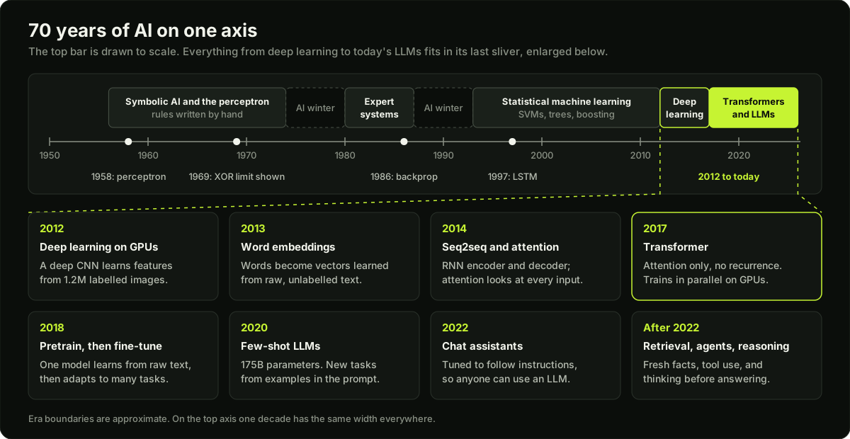 Timeline of AI from 1950 to today with the years since 2012 enlarged into eight steps
AI winters and expert systems
Promises ran ahead of results, and funding collapsed twice: in the mid-1970s and again in the late 1980s. These periods are called AI winters. Between them, the 1980s belonged to expert systems: thousands of if-then rules collected from human specialists, for narrow jobs such as diagnosing faults. They earned money, but every rule was written and maintained by hand, and they broke on any case their authors had not foreseen.
Backpropagation and statistical machine learning
In 1986 backpropagation was shown to train networks with hidden layers: pass the error backward with the chain rule and adjust every weight. That removed the XOR limit. The networks stayed small, though. Datasets were tiny, computers were slow, and gradients faded in deep stacks.
So the 1990s and 2000s went to statistical machine learning: support vector machines (SVMs), decision trees, random forests and boosting. They learn the decision from data, and boosted trees are still a top choice for tables of numbers. Their limit was the input. People had to design the features for each task, such as edge detectors for images or word counts for text.
2012: deep learning works at scale
In 2012 a deep convolutional neural network (CNN) won the main image classification contest with 15.3% top-5 error. The runner-up, built on hand-designed features, scored 26.2%. Three things came together: 1.2 million labelled images, GPUs fast enough to train on them, and training tricks such as ReLU and dropout. The network learned its own features from raw pixels, so the hand-design step disappeared. Two limits remained: it needed very large labelled datasets, and language was still unsolved.
Words, sequences and attention
Word embeddings (2013) gave every word a dense vector learned from raw, unlabelled text. Similar words sit close together, and king - man + woman lands near queen. The limit: one fixed vector per word, so "bank" means the same thing next to "river" and next to "loan".
Sequence-to-sequence models (2014) used one recurrent neural network (RNN) to read a sentence into a single vector and a second one to write the translation. Long sentences did not fit through that one vector. Attention, added the same year, let the decoder look back at every input word at each step. The RNN underneath still read one token at a time, which is slow to train and loses long-range context.
The transformer and pretraining
The transformer (2017) dropped recurrence and kept only attention. Any two tokens connect in one step, and all positions train in parallel on GPUs. Its costs: attention grows with the square of the sequence length, and each task still needed its own labelled data.
Pretraining (2018 onward) fixed the data problem. Train a transformer on raw text to predict hidden or next tokens, then fine-tune it on a small labelled set. Encoder models (BERT style) became the standard for classification and search, decoder models (GPT style) for generation. The limit: one fine-tune per task.
In 2020 a decoder with 175 billion parameters showed that a large enough model can do a new task from a few examples in the prompt, with no weight updates. This is few-shot learning. It was still hard to steer, it made things up, and it knew nothing after its training data ended.
Chat assistants, retrieval, agents and reasoning
Chat assistants (2022) added instruction tuning and alignment from human feedback, so the model follows a plain request. What a chat model still cannot do explains most of today's stack:
- Stale or missing knowledge, invented facts: retrieval-augmented generation (RAG) fetches documents at query time.
- It can only write text: agents let the model call tools in a loop and act on the results.
- Mistakes on multi-step problems: reasoning models think before they answer, trained with reinforcement learning on rewards that can be checked automatically.
Still open: cost, latency, reliability over long tasks, and security.
The chain in one table
| Era | Main idea | What limited it |
|---|---|---|
| 1950s to 1960s: symbolic AI | Hand-written rules and search | Rules cannot cover messy real input |
| 1958: perceptron | Learn weights from examples | One layer: straight-line boundaries only, no XOR |
| 1980s: expert systems | Thousands of rules from specialists | Costly to maintain, brittle outside a narrow domain |
| 1986: backpropagation | Train hidden layers with the chain rule | Little data, slow computers, vanishing gradients |
| 1990s to 2000s: statistical ML | SVMs, trees, boosting | Features designed by hand for every task |
| 2012: deep learning | Deep CNN, GPUs, 1.2 million labelled images | Needs huge labelled sets; text unsolved |
| 2013: word embeddings | Word vectors from raw text | One vector per word, whatever the context |
| 2014: seq2seq and attention | RNN encoder-decoder that looks back at the input | Token by token: slow, forgets long-range context |
| 2017: transformer | Attention only, parallel training | Quadratic cost; labelled data per task |
| 2018: pretraining | Pretrain on raw text, then fine-tune | A separate fine-tune for every task |
| 2020: few-shot LLMs | The task is given in the prompt | Hard to steer, invents facts, frozen knowledge |
| 2022: chat assistants | Tuned to follow instructions | Stale knowledge, text only, weak multi-step reasoning |
| After 2022 | Retrieval, agents, reasoning models | Cost, latency, long-task reliability, security |
Diagram
Worked example
Why one perceptron cannot learn XOR, and how a hidden layer fixes it. This small proof is the first "limit, then idea" step in the chain, and you can do it on paper.
A perceptron outputs 1 when w1 x1 + w2 x2 + b is greater than 0, and 0 otherwise. XOR outputs 1 only when exactly one input is 1. For a perceptron to compute XOR, four conditions must hold:
- Input (0, 0) gives 0, so b is at most 0.
- Input (0, 1) gives 1, so w2 + b is greater than 0.
- Input (1, 0) gives 1, so w1 + b is greater than 0.
- Input (1, 1) gives 0, so w1 + w2 + b is at most 0.
Add conditions 2 and 3: w1 + w2 + 2b is greater than 0, so w1 + w2 + b is greater than -b. Condition 1 says -b is at least 0. So w1 + w2 + b is greater than 0, which contradicts condition 4. No weights exist. In a picture: no single straight line puts (0, 1) and (1, 0) on one side and (0, 0) and (1, 1) on the other.
Now add two hidden units with the same step rule:
- h1 = step(x1 + x2 - 0.5), which is OR
- h2 = step(x1 + x2 - 1.5), which is AND
- output = step(h1 - h2 - 0.5), which is "OR and not AND"
| x1 | x2 | h1 | h2 | h1 - h2 - 0.5 | Output |
|---|---|---|---|---|---|
| 0 | 0 | 0 | 0 | -0.5 | 0 |
| 0 | 1 | 1 | 0 | 0.5 | 1 |
| 1 | 0 | 1 | 0 | 0.5 | 1 |
| 1 | 1 | 1 | 1 | -0.5 | 0 |
All four rows are correct. So a hidden layer has enough capacity. The open problem was how to learn those hidden weights, because the step function has zero slope and gives no signal about which way to move. Smooth activations plus backpropagation (1986) answered that, which is the next link in the chain.
Runnable code
"""Why the field needed hidden layers: a perceptron learns AND but never XOR.

Part 1 trains a single perceptron with the classic learning rule.
Part 2 shows that two hidden units with hand-set weights solve XOR.
"""
import numpy as np

X = np.array([[0, 0], [0, 1], [1, 0], [1, 1]])
AND = np.array([0, 0, 0, 1])
XOR = np.array([0, 1, 1, 0])


def step(z):
    return (z > 0).astype(int)


def train_perceptron(X, y, epochs=100, lr=0.1):
    """Perceptron rule: on each mistake, move the weights toward the example."""
    w, b = np.zeros(2), 0.0
    for epoch in range(1, epochs + 1):
        mistakes = 0
        for xi, target in zip(X, y):
            pred = int(w @ xi + b > 0)
            if pred != target:
                w += lr * (target - pred) * xi
                b += lr * (target - pred)
                mistakes += 1
        if mistakes == 0:                      # a full pass with no mistake: converged
            return w, b, epoch
    return w, b, None


def two_layer_xor(X):
    """Hidden unit 1 computes OR, hidden unit 2 computes AND, output = OR and not AND."""
    h1 = step(X[:, 0] + X[:, 1] - 0.5)         # OR
    h2 = step(X[:, 0] + X[:, 1] - 1.5)         # AND
    return step(h1 - h2 - 0.5)


if __name__ == "__main__":
    for name, y in [("AND", AND), ("XOR", XOR)]:
        w, b, epoch = train_perceptron(X, y)
        acc = (step(X @ w + b) == y).mean()
        status = f"converged in {epoch} epochs" if epoch else "never converged in 100 epochs"
        print(f"perceptron on {name}: {status}, accuracy {acc:.2f}")
        assert (acc == 1.0) == (name == "AND")

    out = two_layer_xor(X)
    print("two-layer network on XOR:", out, "target:", XOR)
    assert (out == XOR).all()
    print("one hidden layer solves XOR; a single perceptron cannot")
Key takeaways
The history is a chain: each method had a clear limit, and the next idea removed it.
Rules and expert systems failed because people had to write every rule. Statistical ML learned the decision but still needed hand-designed features.
Deep learning took off in 2012 when large labelled data, GPUs and better training tricks met. Backpropagation itself dates from 1986.
Attention (2014) was added to RNNs to remove the single-vector bottleneck. The transformer (2017) kept attention and removed the RNN.
Pretraining on raw text removed the need for labelled data per task. Large models then made the prompt the interface.
RAG, agents and reasoning models each answer one limit of a plain chat model: stale knowledge, no actions, weak multi-step reasoning.
Common mistakes
Saying deep learning was invented in 2012. The ideas were decades old; data and GPUs made them work.
Saying the transformer invented attention. Attention came three years earlier, on top of RNNs.
Treating classical ML as obsolete. Boosted trees still win on many tabular problems and cost far less to run.
Reciting dates without the reason. The interviewer wants the limit and the fix, not the year.
Practice
Close the lesson and write the "era, main idea, what limited it" table from memory. Aim for at least 10 of the 13 rows with the correct limit.
Explain aloud, in under two minutes, the path from the perceptron to the transformer. Record it and check that you named at least six "limit, then fix" steps.
Run the code example, then change the target to OR and to NAND. Record how many epochs the perceptron needs for each, and explain why both converge when XOR does not.
Interview questions (6)
1.Why did transformers replace RNNs and LSTMs?Easy
RNNs process tokens one by one, so they cannot be parallelised and they forget long-range context. Attention connects any two tokens directly and trains in parallel on GPUs. To add detail: in an RNN, information from token 1 must survive every step to reach token 100, and the gradient has to travel the same path back, so it fades. LSTMs reduce that with gates but still run step by step. In a transformer the path between any two tokens is one attention step, and a whole sequence is processed in one pass. That made it practical to train on far more text, which is what later made pretraining and LLMs possible. The price is attention cost that grows with the square of the sequence length.
2.Backpropagation dates from 1986. Why did deep learning only take off in 2012?Medium
Three ingredients were missing. Data: deep networks need a lot of labelled examples, and a dataset with over a million labelled images only arrived around 2010. Compute: training on that much data was too slow on CPUs, and GPUs made it many times faster. Training methods: sigmoid networks suffered from vanishing gradients, and ReLU, better initialisation and dropout made deeper stacks trainable. In 2012 all three came together and a deep convolutional network cut the top-5 error on the main image benchmark to 15.3%, against 26.2% for the best system built on hand-designed features. After that result most of the field moved to deep learning.
3.What were the AI winters, and what caused them?Easy
They were two periods, in the mid-1970s and the late 1980s, when funding and interest in AI dropped sharply. Both followed the same pattern: large promises, systems that worked in demos but not on real problems, then disappointment. The first followed the limits of early symbolic AI and of the single-layer perceptron. The second followed expert systems, which were expensive to build and maintain because every rule was written by hand, and which broke outside their narrow domain. The lesson I take from it is to judge a method by measured results on real tasks, which is why I care about evals for LLM systems.
4.What did pretraining change, and how do encoder and decoder models differ?Medium
Before pretraining, each task needed its own model trained on its own labelled data. Pretraining trains one transformer on raw text with a self-supervised objective, so the labels come for free from the text itself. The model learns general language knowledge once, and a small labelled set is enough to adapt it. Encoder models hide some tokens and predict them using context on both sides, so they produce good representations for classification, search and reranking. Decoder models predict the next token using only the left context, so they generate text. Scaling up decoders led to few-shot LLMs, where the task is described in the prompt and no fine-tune is needed.
5.Which limits of a plain LLM led to RAG, agents and reasoning models?Medium
A plain LLM only knows its training data, so it is out of date, it has never seen private documents, and it fills gaps with fluent guesses. RAG addresses that by retrieving relevant text at query time and putting it in the prompt. A plain LLM also only produces text. Agents address that by letting the model call tools in a loop: search, run code, call an API, then read the result and decide the next step. Finally, a model that answers in one pass makes mistakes on multi-step problems. Reasoning models spend tokens thinking before the answer. What is still open is cost, latency, reliability over long tasks and security.
6.Are classical ML models still worth knowing now that LLMs exist?Easy
Yes. For structured tables with numeric and categorical columns, such as fraud scores, credit risk or click prediction, gradient-boosted trees are often the most accurate option, and they often train in minutes on a CPU. They are cheap to serve and easier to explain. Logistic regression is still the usual baseline and the final layer of many systems. LLMs are the right tool for open-ended language tasks. A common production design uses both: a small classical model or small neural model for high-volume narrow decisions, and an LLM for the cases that need language understanding.
Quiz
1.What limit of the single-layer perceptron was shown in 1969?
2.What did statistical ML methods such as SVMs and boosted trees still depend on people for?
3.Which three things came together in the 2012 image classification result?
4.What problem did the first attention mechanism (2014) solve?
5.A model answers a question about last week's news with an invented fact. Which later idea targets this limit most directly?
Practice these problems
Further reading
My notes
Your notes
Autosaves to this browser.