Neural networks and backprop
A neural network is a stack of simple units. Each unit multiplies its inputs by weights, adds a bias and applies a non-linear function. Training means finding weights that make a loss number small. Backpropagation computes how much each weight contributed to the loss, and gradient descent moves each weight a small step in the direction that lowers it. This lesson covers both, plus the basics interviewers check: activations, losses, optimisers, regularisation, normalisation and metrics.
Why it matters
Every LLM is a neural network trained with backpropagation, so this is the floor under every other lesson. Many AI engineer interview loops include a round on ML and deep learning basics: bias and variance, regularisation, optimisers, backpropagation, loss functions and classification metrics. The questions are short ("why cross-entropy?", "why does Adam work?", "validation loss is rising, what now?") and the interviewer expects a precise answer in under a minute. You also need this to read a training curve, to debug a fine-tune that does not converge, and to write the from-scratch coding problems on this site.
Lesson
A neuron: weights, bias, activation
A neuron takes a list of numbers, multiplies each by a weight, adds them up with a bias, and passes the result through an activation function.
With inputs x = [1, 2], weights w = [0.5, -0.25] and bias b = 0.1, z = 0.5 - 0.5 + 0.1 = 0.1. The weights say how much each input matters. The bias shifts the point where the neuron switches on. Weights and biases are the parameters, the numbers that training changes.
Activation functions and why non-linearity is needed
Without an activation function, two layers collapse into one: W2(W1 x) = (W2 W1) x, which is still a single matrix. A stack of 100 linear layers can only draw straight-line boundaries. The non-linear function between layers is what lets a network fit curves, and XOR is the smallest example a linear model cannot fit.
| Activation | Formula | Output range | Where it is used |
|---|---|---|---|
| ReLU | max(0, z) | 0 to infinity | Default for hidden layers; slope is 1 or 0, so it is cheap and gradients survive |
| Sigmoid | 1 / (1 + e^-z) | 0 to 1 | Binary output, gates in LSTMs; slope is at most 0.25 |
| Tanh | (e^z - e^-z) / (e^z + e^-z) | -1 to 1 | RNN hidden states; centred on zero, slope at most 1 |
| GELU | z times the normal CDF of z | about -0.17 to infinity | Transformers; a smooth version of ReLU |
| Softmax | e^z_k / sum of e^z_j | each 0 to 1, sum is 1 | Output layer for multi-class problems, and attention weights |
Softmax turns logits (raw scores) into probabilities. Logits [2, 1, 0] become [0.665, 0.245, 0.090]: every gap of 1 in the logits is a factor of e, about 2.72, in probability.
A ReLU unit whose input is always negative outputs 0 and gets zero gradient, so it never recovers. This is the "dead ReLU" problem. Leaky ReLU and GELU reduce it by keeping a small non-zero slope for negative inputs.
Layers and the forward pass
A layer is many neurons that share the same inputs, written as one matrix multiply. A two-layer network is:
Computing the output from the input is the forward pass. Count parameters layer by layer. A network with 784 inputs, 128 hidden units and 10 outputs has 784 x 128 + 128 = 100,480 parameters in the first layer and 128 x 10 + 10 = 1,290 in the second: 101,770 in total. The raw outputs before softmax are called logits.
Loss functions
The loss is one number that says how wrong the predictions are. Training minimises it.
- Mean squared error (MSE) is the average of (prediction - target)^2. Use it for regression.
- Cross-entropy is for classification. With a one-hot label (1 for the correct class, 0 for the others) it is the negative log of the probability given to the correct class.
If the model gives the correct class probability 0.7, the loss is -ln 0.7 = 0.357. At 0.01 it is 4.605. Confident wrong answers are punished hard. With softmax or sigmoid outputs, the gradient of cross-entropy with respect to the logits is simply p - y. MSE on a sigmoid output multiplies the gradient by the sigmoid slope, which is near zero when the model is confidently wrong, so learning stalls exactly when it should be fastest.
Gradient descent, learning rate and mini-batches
The gradient of the loss with respect to a weight says which way the loss rises. Step the other way:
The learning rate (eta) is the step size. Too small and training takes forever. Too large and the loss jumps around or diverges. It is the first hyperparameter (a setting you choose, not one the model learns) to tune. Most training runs warm it up from near zero for the first steps and then decay it.
- Batch gradient descent uses the whole dataset for each step: exact but slow.
- Stochastic gradient descent (SGD) uses one example: fast but noisy.
- Mini-batch SGD uses 32 to 512 examples: a good estimate of the gradient, and one GPU matrix multiply per batch. This is what everyone uses.
One pass over the training set is an epoch. The noise from small batches also helps a little against overfitting.
Backpropagation
Backpropagation is the chain rule applied to the computation graph, from the loss back to the inputs. The forward pass stores every intermediate value. The backward pass starts with the gradient 1 at the loss and visits the nodes in reverse order. Each node multiplies the gradient it receives by its local slope and passes the result on.
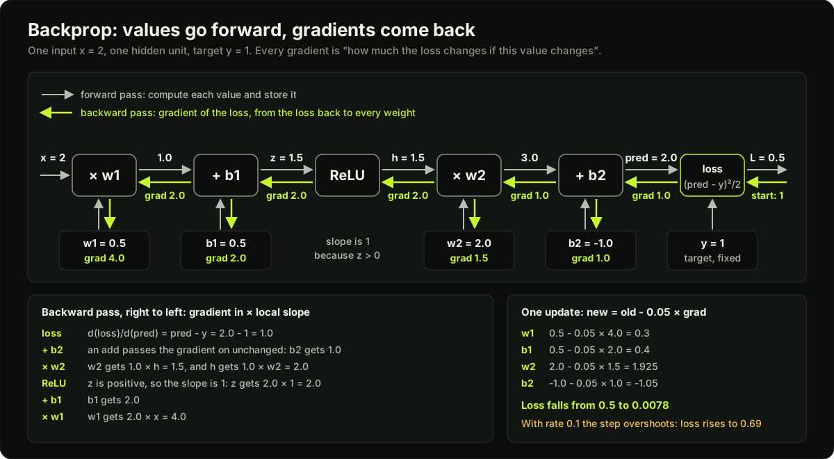 Computation graph of a one-hidden-unit network with forward values above each arrow and gradients below
Three local rules cover most networks. An add node passes the gradient through unchanged. A multiply node gives each input the gradient times the other input. An activation multiplies by its slope at the stored value. For a two-layer network with a batch X this becomes four lines:
One backward pass costs about the same as one forward pass and gives the gradient for every weight at once. That is why training networks with billions of weights is possible. Frameworks do this automatically (autograd), but interviewers still ask you to derive it for a small network.
Initialisation, vanishing and exploding gradients
If all weights start at zero, every neuron in a layer computes the same output and gets the same gradient, so they stay identical for ever. Start with small random values, scaled so the signal keeps roughly the same variance from layer to layer:
- Xavier initialisation: variance 2 / (fan_in + fan_out). Use with tanh and sigmoid.
- He initialisation: variance 2 / fan_in. Use with ReLU, which zeroes half its inputs.
Here fan_in is the number of inputs to a unit and fan_out is the number of units its output feeds.
The backward pass multiplies one factor per layer. If the factors are below 1 the gradient shrinks: the slopes of ten sigmoid layers multiply to at most 0.25^10, about 0.000001, so early layers stop learning. This is the vanishing gradient problem. Fixes: ReLU-family activations, correct initialisation, normalisation layers, and residual connections (output = x + F(x)), which give the gradient a direct path around each block. If the factors are above 1 the gradient explodes and the loss becomes NaN (not a number). Fix it with gradient clipping (rescale the gradient when its norm passes a limit such as 1.0) and a lower learning rate.
Overfitting, bias and variance
Bias is the error from a model too simple to capture the pattern. Variance is the error from a model that fits the noise in its particular training set. You diagnose them from two numbers.
| Training error | Validation error | Diagnosis | What to try |
|---|---|---|---|
| High | High | High bias (underfitting) | Bigger model, train longer, better features, less regularisation |
| Low | High | High variance (overfitting) | More data, regularisation, smaller model, early stopping |
| Low | Low | Good fit | Stop and check the test set |
Regularisation is anything that reduces overfitting:
- L2 (weight decay): add lambda times the sum of squared weights to the loss. Large weights are pulled toward zero and the function becomes smoother. L1 uses absolute values and pushes weights to exactly zero.
- Dropout: during training, set each activation to zero with probability p (0.1 to 0.5) and divide the rest by 1 - p. The network cannot rely on any single unit. Turn it off at inference.
- Early stopping: track the validation loss and keep the checkpoint (a saved copy of the weights) where it was lowest.
- More data, real or augmented, is the most reliable fix.
Optimisers
- SGD with momentum keeps a running average of past gradients: v = beta x v + g, then w = w - eta x v, with beta = 0.9. It speeds up along directions where gradients agree and damps zig-zags.
- Adam keeps a running average of the gradient (m) and of the squared gradient (v), corrects both for starting at zero, and divides one by the square root of the other. Each weight gets its own step size: a weight with small gradients takes relatively larger steps. Defaults: beta1 = 0.9, beta2 = 0.999, learning rate 0.001.
- AdamW applies weight decay directly to the weights and not through the gradient. It is the usual choice for transformers.
Here the hats mean bias-corrected: m divided by (1 - beta1^t) and v divided by (1 - beta2^t). Epsilon is a tiny constant, 1e-8 by default, that prevents division by zero. Adam works with little tuning. SGD with momentum needs a tuned learning-rate schedule but is still common for vision models.
Batch norm vs layer norm
Normalisation layers rescale activations to mean 0 and variance 1, then apply a learned scale and shift. They keep signals in a stable range, so deeper networks train with larger learning rates.
| Batch norm | Layer norm | |
|---|---|---|
| Statistics taken over | The batch, per feature | The features, per example |
| Depends on batch size | Yes; small batches give noisy statistics | No |
| Train vs inference | Different: uses stored running averages at inference | Same |
| Typical use | CNNs | Transformers, RNNs |
Transformers use layer norm because sequences have different lengths and batch statistics over padded tokens are unreliable.
Train, validation and test splits
Split the data once, for example 80 / 10 / 10. Fit weights on the training set. Choose hyperparameters and the early-stopping point on the validation set. Touch the test set once, at the end, to report the final number. If you tune on the test set, its score no longer tells you how the model does on new data. Watch for leakage: split by user or by time when rows are related, and compute scaling statistics on the training set only.
Classification metrics
Count four outcomes: true positives (TP), false positives (FP), false negatives (FN), true negatives (TN).
| Metric | Formula | Question it answers |
|---|---|---|
| Accuracy | (TP + TN) / all | How often is the model right? |
| Precision | TP / (TP + FP) | When it says positive, how often is it right? |
| Recall | TP / (TP + FN) | Of the real positives, how many did it find? |
| F1 | 2PR / (P + R) | One number that is low if either precision or recall is low |
| ROC-AUC | Area under the curve of true positive rate vs false positive rate | How well do the scores rank positives above negatives, over all thresholds? |
Take 1,000 transactions with 10 frauds. A model flags 20 and 8 of them are fraud. Precision = 8 / 20 = 0.40, recall = 8 / 10 = 0.80, F1 = 0.53, accuracy = 986 / 1,000 = 0.986. A model that never flags anything scores 0.99 accuracy and finds no fraud. On imbalanced data, report precision and recall, not accuracy. In the ROC curve, the true positive rate is recall and the false positive rate is FP / (FP + TN). ROC-AUC equals the chance that a random positive gets a higher score than a random negative: 0.5 is random, 1.0 is perfect. Moving the decision threshold trades precision for recall.
Diagram
Worked example
One full training step by hand. The network has one input, one hidden ReLU unit and one linear output. Start with x = 2, target y = 1, w1 = 0.5, b1 = 0.5, w2 = 2.0, b2 = -1.0. The loss is half the squared error.
Forward pass. Store every value.
- z = w1 x + b1 = 0.5 x 2 + 0.5 = 1.5
- h = ReLU(1.5) = 1.5
- pred = w2 h + b2 = 2.0 x 1.5 - 1.0 = 2.0
- L = 0.5 x (2.0 - 1)^2 = 0.5
Backward pass. Start at the loss and move left. Each line is "gradient arriving times local slope".
- dL/dpred = pred - y = 1.0
- dL/db2 = 1.0 (an add passes the gradient through)
- dL/dw2 = 1.0 x h = 1.5
- dL/dh = 1.0 x w2 = 2.0
- dL/dz = 2.0 x 1 = 2.0 (ReLU slope is 1 because z is positive)
- dL/db1 = 2.0
- dL/dw1 = 2.0 x x = 4.0
Update with learning rate 0.05. w1 = 0.5 - 0.05 x 4.0 = 0.3. b1 = 0.5 - 0.05 x 2.0 = 0.4. w2 = 2.0 - 0.05 x 1.5 = 1.925. b2 = -1.0 - 0.05 x 1.0 = -1.05.
Check that the loss fell. z = 0.3 x 2 + 0.4 = 1.0, h = 1.0, pred = 1.925 - 1.05 = 0.875, L = 0.5 x 0.125^2 = 0.0078. The loss dropped from 0.5 to 0.0078 in one step.
Same gradients, learning rate 0.1. w1 = 0.1, b1 = 0.3, w2 = 1.85, b2 = -1.1. Then z = 0.5, h = 0.5, pred = 0.925 - 1.1 = -0.175 and L = 0.5 x 1.175^2 = 0.69. The step was in the right direction but too long, and the loss is now higher than where it started. The gradient only describes the slope at the current point, which is why the learning rate matters so much.
Sanity check. Nudge w1 to 0.501 and recompute: z = 1.502, pred = 2.004, L = 0.5 x 1.004^2 = 0.504008. The loss moved by 0.004008 for a nudge of 0.001, a slope of about 4.0, which matches dL/dw1.
Runnable code
"""A two-layer network that learns XOR, with backprop written by hand.

Shapes: X (4, 2) -> hidden (4, 4) with tanh -> output (4, 1) with sigmoid.
Loss: binary cross-entropy. A numerical gradient check proves the backward pass.
"""
import numpy as np

X = np.array([[0, 0], [0, 1], [1, 0], [1, 1]], dtype=np.float64)
Y = np.array([[0], [1], [1], [0]], dtype=np.float64)


def init_params(hidden=4, seed=0):
    rng = np.random.default_rng(seed)
    return {
        # Xavier initialisation: std = sqrt(2 / (fan_in + fan_out))
        "W1": rng.normal(0, np.sqrt(2 / (2 + hidden)), (2, hidden)),
        "b1": np.zeros(hidden),
        "W2": rng.normal(0, np.sqrt(2 / (hidden + 1)), (hidden, 1)),
        "b2": np.zeros(1),
    }


def forward(p, X):
    z1 = X @ p["W1"] + p["b1"]          # (4, hidden)
    h = np.tanh(z1)                     # hidden activations
    z2 = h @ p["W2"] + p["b2"]          # (4, 1) logits
    y_hat = 1 / (1 + np.exp(-z2))       # sigmoid: probability of class 1
    return y_hat, h


def bce(y_hat, Y):
    return float(-np.mean(Y * np.log(y_hat) + (1 - Y) * np.log(1 - y_hat)))


def backward(p, X, Y):
    """Return the loss and dLoss/dparam for every parameter (chain rule, back to front)."""
    y_hat, h = forward(p, X)
    n = len(X)
    d_z2 = (y_hat - Y) / n              # sigmoid + cross-entropy simplify to (p - y)
    d_h = d_z2 @ p["W2"].T              # send the gradient back through W2
    d_z1 = d_h * (1 - h ** 2)           # tanh slope is 1 - tanh(z)^2
    grads = {
        "W2": h.T @ d_z2, "b2": d_z2.sum(axis=0),
        "W1": X.T @ d_z1, "b1": d_z1.sum(axis=0),
    }
    return bce(y_hat, Y), grads


def gradient_check(p, X, Y, eps=1e-5):
    """Compare backprop with (L(w + eps) - L(w - eps)) / (2 eps) for every weight."""
    _, grads = backward(p, X, Y)
    worst = 0.0
    for name, arr in p.items():
        for idx in np.ndindex(arr.shape):
            old = arr[idx]
            arr[idx] = old + eps
            plus = bce(forward(p, X)[0], Y)
            arr[idx] = old - eps
            minus = bce(forward(p, X)[0], Y)
            arr[idx] = old
            numeric = (plus - minus) / (2 * eps)
            analytic = grads[name][idx]
            rel = abs(numeric - analytic) / max(1e-12, abs(numeric) + abs(analytic))
            worst = max(worst, rel)
    return worst


if __name__ == "__main__":
    params = init_params()
    worst = gradient_check(params, X, Y)
    print(f"gradient check: worst relative error = {worst:.2e}")
    assert worst < 1e-6, "backward pass is wrong"
    print("gradient check passed")

    lr = 1.0
    for step in range(2001):
        loss, grads = backward(params, X, Y)
        if step in (0, 50, 100, 200, 500, 1000, 2000):
            print(f"step {step:4d}  loss {loss:.4f}")
        for name in params:
            params[name] -= lr * grads[name]      # plain gradient descent on the full batch

    y_hat, _ = forward(params, X)
    print("predictions:", np.round(y_hat.ravel(), 3), "targets:", Y.ravel().astype(int))
    assert np.array_equal((y_hat > 0.5).astype(int), Y.astype(int))
    print("XOR learned: all 4 points classified correctly")
Key takeaways
A neuron computes f(w . x + b). Without the non-linear f, any stack of layers is one linear layer.
Backprop is the chain rule on the computation graph: one forward pass to store values, one backward pass to get every gradient, at about the cost of the forward pass.
Gradient descent is w = w - learning rate x gradient. The learning rate is the first thing to tune; mini-batches of 32 to 512 are the norm.
Use cross-entropy for classification. With softmax or sigmoid its gradient at the logits is p - y.
Vanishing gradients come from multiplying many slopes below 1. ReLU, He or Xavier initialisation, normalisation and residual connections fix it; clipping handles exploding gradients.
High training error means bias; low training error with high validation error means variance. L2, dropout, early stopping and more data reduce variance.
Adam adapts the step per weight and needs little tuning; AdamW is the usual choice for transformers.
On imbalanced data report precision, recall and F1, not accuracy. ROC-AUC measures ranking over all thresholds.
Common mistakes
Saying "backprop updates the weights". Backprop only computes gradients; the optimiser does the update.
Leaving dropout or batch norm in training mode at inference, which makes outputs random or batch-dependent.
Tuning hyperparameters on the test set and then reporting the test score as unbiased.
Using accuracy on a dataset where 99% of rows are one class.
Applying softmax in the model and again inside the loss function, which flattens the gradients.
Forgetting to shuffle the training data each epoch, so every batch has the same biased mix.
Practice
Run the code example, then change the hidden activation from tanh to ReLU. Update the backward pass, and start b1 at 0.1: with b1 = 0 the input (0, 0) puts every hidden unit exactly on the ReLU kink, where a numerical check is not valid. Make the gradient check pass again with a worst relative error below 1e-6.
Redo the worked example on paper with x = 3 and target y = 0. Write down all four gradients, then confirm them by nudging each weight by 0.001 in a five-line script.
Train the XOR network with learning rates 0.01, 0.1, 1 and 10 for 2,000 steps each. Record the final loss for each and explain the two failures.
For a classifier that outputs scores, compute precision, recall and F1 at thresholds 0.3, 0.5 and 0.7 on 20 hand-made examples, and say which threshold you would ship for a fraud alert and why.
Interview questions (14)
1.Explain backpropagation.Medium
Backpropagation computes the gradient of the loss with respect to every weight using the chain rule. First a forward pass computes the output and stores each intermediate value. Then a backward pass starts at the loss and walks the computation graph in reverse. Each node takes the gradient arriving from the right, multiplies it by its own local derivative, and passes it left. An add passes the gradient through, a multiply scales it by the other input, an activation scales it by its slope. Because intermediate results are reused, one backward pass gives all the gradients for about the cost of one forward pass. The optimiser then uses those gradients to update the weights.
2.Why do neural networks need non-linear activation functions?Easy
Because a stack of linear layers is still one linear layer. Multiplying by W1 and then by W2 is the same as multiplying by the single matrix W2 W1, so depth adds nothing and the model can only learn straight-line boundaries. A non-linear function between layers breaks that collapse. With it, each layer can bend the space a little and the stack can approximate very complicated functions. XOR is the standard example: no single line separates its classes, but one hidden layer with a non-linearity solves it.
3.Why cross-entropy and not mean squared error for classification?Medium
Two reasons. First, cross-entropy matches the problem: it is the negative log-likelihood of the correct class, so minimising it makes the predicted probabilities as close as possible to the labels. Second, the gradients are better. With a sigmoid or softmax output, the gradient of cross-entropy with respect to the logit is just p minus y, which is large when the model is confidently wrong. With MSE the gradient is also multiplied by the sigmoid slope, which is near zero when the output is saturated near 0 or 1. So a confidently wrong model learns slowly with MSE and quickly with cross-entropy.
4.What are vanishing and exploding gradients, and how do you fix them?Medium
In the backward pass the gradient is multiplied by one factor per layer: the weight matrix and the activation slope. If those factors are mostly below 1, the product shrinks toward zero and the early layers stop learning. That is vanishing. Sigmoid makes it worse because its slope is at most 0.25. If the factors are above 1 the product blows up and the loss becomes NaN. That is exploding. For vanishing I use ReLU-family activations, He or Xavier initialisation, normalisation layers and residual connections, which give the gradient a direct path. For exploding I clip the gradient norm and lower the learning rate. LSTMs solve the same problem across time steps with a cell state that is updated by addition.
5.Explain the bias-variance trade-off.Easy
Bias is error from a model that is too simple, so it misses the real pattern even on the training data. Variance is error from a model that is too sensitive to its particular training set, so it fits noise and does badly on new data. Making a model larger usually lowers bias and raises variance. In practice I read it from two numbers: high training error means bias, so I increase capacity or train longer. Low training error with a much higher validation error means variance, so I add data, regularisation or early stopping. Large pretrained networks complicate the classical picture, but the diagnostic still works.
6.L1 vs L2 regularisation?Medium
Both add a penalty on weight size to the loss. L2 adds the sum of squared weights. Its gradient is proportional to the weight, so big weights shrink fast and small ones shrink slowly; weights get small but rarely exactly zero. L1 adds the sum of absolute values. Its gradient is a constant push toward zero, so many weights end at exactly zero, which gives a sparse model and acts as feature selection. L2, usually as weight decay, is the default for neural networks. One detail worth saying: with Adam, weight decay should be applied directly to the weights, which is what AdamW does.
7.How does dropout work, and what changes at inference?Medium
During training, dropout sets each activation to zero with probability p, chosen fresh for every example and step. The network cannot depend on any single unit, so it spreads information across many units, which reduces overfitting. It behaves a bit like training many smaller networks that share weights. To keep the expected activation the same, the surviving units are divided by 1 minus p. At inference dropout is switched off and all units are used, with no extra scaling needed. A common bug is forgetting to switch the model to evaluation mode, which leaves dropout on and makes predictions noisy.
8.SGD with momentum vs Adam: how do they differ and when do you use each?Medium
SGD with momentum keeps a running average of past gradients and steps along it, which speeds up consistent directions and damps oscillation. It uses one learning rate for all weights. Adam also keeps a running average of the squared gradient and divides the step by its square root, so each weight gets its own effective learning rate: weights with small or rare gradients take larger steps. Adam also corrects both averages for starting at zero. Adam, usually AdamW, converges fast with little tuning and is the standard for transformers. SGD with momentum needs a carefully tuned schedule but often does as well or better on vision models.
9.Batch norm vs layer norm, and why do transformers use layer norm?Medium
Both rescale activations to zero mean and unit variance and then apply a learned scale and shift. Batch norm computes the statistics for each feature across the batch, so it depends on batch size and must store running averages to use at inference. Layer norm computes them across the features of a single example, so it behaves the same in training and inference and works with a batch of one. Transformers use layer norm because text batches contain sequences of different lengths with padding, and generation runs token by token, so batch statistics are unreliable. Many LLMs place the norm before each sub-layer, which trains more stably in deep stacks.
10.Precision vs recall: when do you prefer each, and what does ROC-AUC tell you?Easy
Precision is the share of predicted positives that are correct. Recall is the share of real positives that were found. I optimise precision when a false alarm is expensive, such as blocking a legitimate payment or marking a good email as spam. I optimise recall when a miss is expensive, such as a cancer screen or a safety filter. F1 combines them when I need one number. ROC-AUC is threshold-free: it is the probability that a random positive gets a higher score than a random negative, so it measures ranking quality. On heavily imbalanced data I prefer the precision-recall curve, because ROC-AUC can look good while precision is poor.
11.Training loss keeps falling but validation loss starts rising. What do you do?Medium
That is overfitting: the model has begun to memorise the training set. First I keep the checkpoint with the lowest validation loss, which is early stopping. Then I reduce variance: more or augmented data, stronger weight decay, dropout, or a smaller model. I also check the data: a validation set from a different distribution, or duplicates between train and validation, produce misleading curves. If validation loss rises while validation accuracy still improves, the model is becoming over-confident on its mistakes, so I would look at calibration and not stop on loss alone.
12.Why can you not initialise all weights to zero?Easy
With identical weights, every neuron in a layer computes the same output and receives the same gradient, so after each update they are still identical. The layer behaves like a single neuron however wide it is. This is called the symmetry problem, and random initialisation breaks it. The scale of the random values matters too: too small and signals vanish through the layers, too large and they explode. Xavier initialisation for tanh and He initialisation for ReLU pick the variance from the layer's size (its fan-in, and for Xavier also its fan-out) so the signal keeps a steady size. Biases can start at zero.
13.How would you verify a backward pass you wrote by hand?Hard
With a numerical gradient check. For each parameter I add a small epsilon, compute the loss, subtract epsilon, compute the loss again, and take the difference divided by two epsilon. That central difference approximates the true derivative. I compare it with the backprop value using relative error: the absolute difference divided by the sum of the magnitudes. In float64 with epsilon around 1e-5 a correct implementation gives about 1e-7 or smaller; 1e-2 means a bug. I run it on a tiny network with a few examples, with dropout off, because the check needs one forward pass per parameter. I also overfit a single small batch to confirm the loss goes to near zero.
14.Your training loss is not decreasing, or it becomes NaN. How do you debug it?Hard
I start with the smallest test: can the model overfit one batch of 8 examples? If not, the bug is in the code, not the data size. I check that labels line up with inputs, that the loss matches the output layer (no double softmax), and that gradients are non-zero for every layer. For NaN, I look for an exploding gradient or a log of zero: I lower the learning rate by ten times, add gradient clipping and warmup, and add a small epsilon inside logs and divisions. For a flat loss I try a higher learning rate, check initialisation and look for dead ReLUs. Logging the gradient norm per layer usually points to the problem.
Quiz
1.A network has 3 layers and no activation functions. What can it represent?
2.In a multiply node c = a x b, the gradient arriving at c is 3, a = 2 and b = 5. What gradient does a receive?
3.Training error is 2% and validation error is 19%. Which change is most likely to help?
4.Out of 100 emails, 20 are spam. A filter flags 10 emails and 9 of them are spam. What are precision and recall?
5.Which statement about batch norm and layer norm is correct?
6.Why does Adam often need less learning-rate tuning than plain SGD?
Practice these problems
Further reading
My notes
Your notes
Autosaves to this browser.