LLM fundamentals - tokens, embeddings, decoding
An LLM (large language model) is a neural network trained to do one thing: predict the next token. This lesson follows a piece of text through the whole machine. Text becomes tokens, tokens become vectors, a stack of transformer blocks mixes those vectors, and a decoding rule picks the next token from the output probabilities. You will work each stage with small numbers.
Why it matters
Most GenAI interviews open here. "What is a token?", "Explain self-attention simply", "Temperature vs top-p?" and "Why do LLMs hallucinate?" are warm-up questions, and a weak answer colours the rest of the round. The same ideas decide real engineering work: token counts set your bill and your latency, the context window sets how much history and retrieved text fits, and decoding settings decide whether an extraction job returns the same JSON twice. If you can draw the next-token loop and one transformer block from memory, the later topics (RAG, fine-tuning, serving) become details added to a picture you already have.
Read first: Neural networks and backprop
Lesson
One objective: predict the next token
An LLM is a neural network trained to predict the next token. Chat, code and reasoning all come from that one objective, trained at very large scale.
At run time the model works in a loop. Text is split into tokens. The network outputs a probability for every token in its vocabulary. One token is chosen and appended to the input, and the loop runs again until a stop token appears. Every section below is one stage of that loop.
Run naively, each pass would recompute the whole sequence to produce one token. Real servers keep a KV cache: the attention keys and values of earlier tokens (defined in the self-attention section below) are stored, so each step computes only the new token.
Tokens and BPE
A token is the unit the model reads, usually a word piece. Roughly 1 token is 0.75 English words, so 1,000 tokens is about 750 words.
Why word pieces? A vocabulary of whole words can never cover every name, typo and new word. Single characters cover everything but make sequences very long. Word pieces sit between the two: a common word is one token, and a rare word splits into a few known pieces.
Tokenizers such as BPE (byte pair encoding) build a vocabulary by repeatedly merging the most frequent character pairs:
- Start with every word split into single characters.
- Count every adjacent pair of symbols across the corpus.
- Merge the most frequent pair into one new symbol and add it to the vocabulary.
- Repeat until the vocabulary reaches the size you want.
Here is a tiny corpus, as word counts: play 5, plays 3, played 4, player 2, day 7, plan 2.
| Merge | Most frequent pair | Count | New token | "played" is now |
|---|---|---|---|---|
| 1 | a + y | 21 | ay | p l ay e d |
| 2 | p + l | 16 | pl | pl ay e d |
| 3 | pl + ay | 14 | play | play e d |
| 4 | d + ay | 7 | day | play e d |
Check merge 1: "ay" occurs in play, plays, played, player and day, so 5 + 3 + 4 + 2 + 7 = 21. After four merges the unseen word "replay" encodes as r, e, play: three tokens and no "unknown word" symbol. To encode new text you apply the merges in the order they were learned. Real tokenizers run tens of thousands of merges and usually start from bytes, so any string can be encoded.
Two practical effects follow. The 0.75 ratio is for English prose: code and text in other languages usually need more tokens per word, so measure with the real tokenizer. And the model sees pieces, not letters, which is why "how many r's are in strawberry" is harder for it than it looks.
The embedding table
A token ID is only an index, so the model needs numbers it can do maths on. The embedding table is a matrix with one row per vocabulary entry and d_model columns, where d_model is the length of every token vector inside the model. Token ID 4,821 selects row 4,821. That row is the token's vector, called its embedding.
The rows are learned during training. Tokens that appear in similar contexts end up with similar rows, so similar meanings sit close together in that vector space.
The table gives one fixed vector per token. "bank" gets the same row in "river bank" and "bank loan". It is the transformer blocks that mix in the neighbours and turn this fixed vector into one that fits the sentence.
The table is large. With a vocabulary of 50,000 and d_model = 4,096 it holds 50,000 x 4,096 = 204.8 million parameters. At the other end of the network, an output layer maps the final vector back to 50,000 scores called logits, one per vocabulary token.
Position
Attention has no sense of order: shuffle the input tokens and each token still gets the same result. "Dog bites man" and "man bites dog" would look identical, so position is added.
| Method | How it works | Note |
|---|---|---|
| Sinusoidal | Fixed sine and cosine waves of different frequencies, added to the token embedding | No parameters; used in the original transformer |
| Learned | One trainable vector per position, added to the token embedding | Simple; cannot go past the longest position seen in training |
| Rotary (RoPE) | Rotates query and key vectors by an angle that depends on position, inside every attention layer | The attention score depends on the distance between two tokens; most modern LLMs use it |
RoPE stands for rotary position embeddings. Because both the query and the key are rotated, their dot product depends on the difference of the two angles. The model learns "three tokens back", not "position 507".
Self-attention
Self-attention is the step where tokens exchange information. Every token looks at every other token and decides how much each one matters. It builds a query, a key and a value per token. The query is compared with every key, and the scores decide how much of each value to take.
In a generating model a causal mask hides later tokens, so a token attends only to itself and what came before. The next lesson builds this formula step by step with numbers.
The transformer block
A transformer block is multi-head attention, then a feed-forward layer, each wrapped in a residual connection and layer norm.
- Multi-head attention moves information between tokens. Several attention heads run in parallel.
- Feed-forward layer: two linear layers with a non-linearity between them, applied to each token on its own. It typically expands the vector to about 4 x
d_modeland brings it back. - Residual connection: the input of a sub-layer is added to its output, x + f(x). Gradients get a direct path through the whole stack.
- Layer norm: rescales each token's vector to zero mean and unit variance, which keeps values in a stable range.
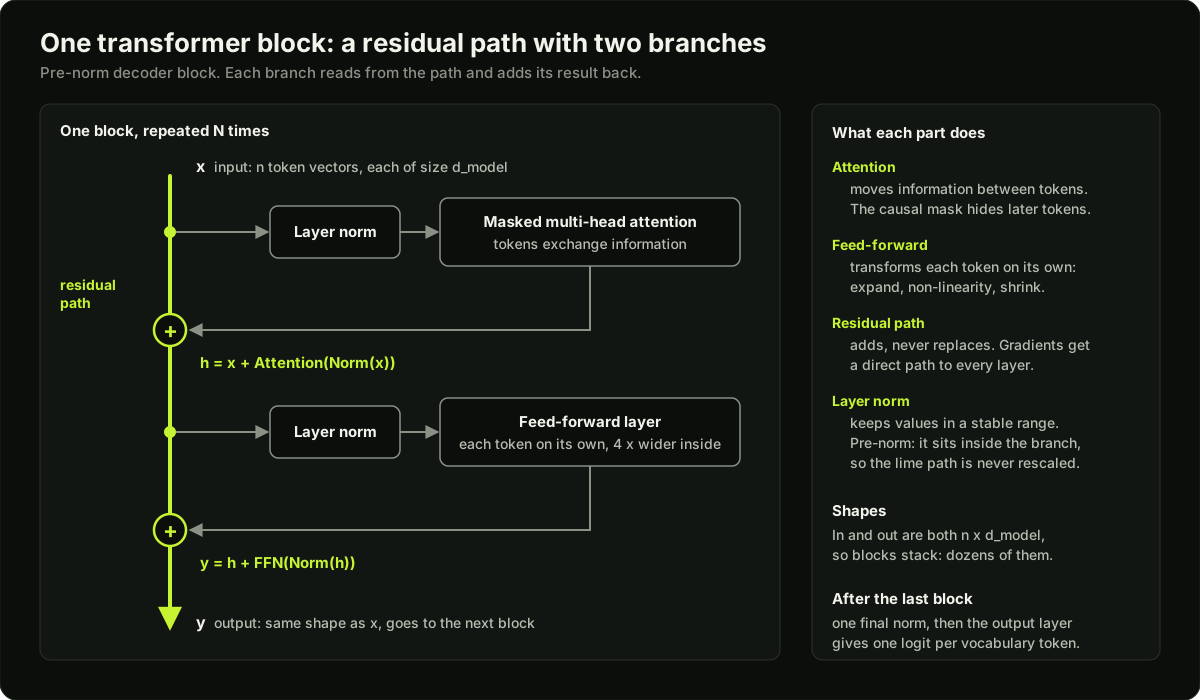 One pre-norm decoder block: a residual path with an attention branch and a feed-forward branch
This order is called pre-norm: normalise first, then run the sub-layer. The original transformer used post-norm, Norm(x + f(x)). Most modern LLMs use pre-norm because the residual path is never rescaled, and deep stacks train more stably. The input and output have the same shape, so you stack dozens of blocks.
Where do the parameters sit? Attention has four d_model x d_model matrices (query, key, value, output), so 4 x d_model^2. A feed-forward layer with 4 x expansion has two matrices of size d_model x 4 d_model, so 8 x d_model^2. With d_model = 4,096 that is about 67 million for attention and 134 million for the feed-forward layer: two thirds of a block's parameters are in the feed-forward part.
Three architectures
| Architecture | What each token sees | One use |
|---|---|---|
| Decoder-only (GPT style) | Causal mask: only earlier tokens | Generation: chat and code |
| Encoder-only (BERT style) | Both directions | Embeddings and classification |
| Encoder-decoder (T5 style) | The encoder reads the input in both directions; the decoder generates and attends to the encoder output | Translation and summarisation |
Most LLMs today are decoder-only.
Training stages
- Pretraining on raw text (next-token prediction). The label is the next token of the text itself, so no human labelling is needed. The loss at each position is the negative log of the probability given to the correct token: 0.69 if the model gave it 0.5, and 4.6 if it gave it 0.01. With a causal mask, a 1,000-token text gives 999 predictions in one pass. The result is a base model that continues text.
- Supervised fine-tuning on instructions. Instruction and response pairs teach the model to answer a request, not just continue it.
- Preference alignment (RLHF or DPO). RLHF is reinforcement learning from human feedback. DPO is direct preference optimisation. Both use human choices between two answers to push the model toward the preferred one.
Reasoning models add reinforcement learning with verifiable rewards: the model is rewarded when a program can check the result, such as a correct final number or passing unit tests.
Decoding
The model outputs a probability for every token. Decoding is the rule that picks one.
| Method | What it does | Effect |
|---|---|---|
| Greedy | Picks the top token | No random choice; can repeat itself |
| Temperature T | Divides the logits by T before softmax | T below 1 sharpens the distribution, T above 1 flattens it |
| Top-k | Keeps the k most likely tokens | Cuts the tail at a fixed size |
| Top-p (nucleus) | Keeps the smallest set whose probability adds up to p | The set shrinks when the model is confident and grows when it is unsure |
Here z is the logit vector. A common order is: apply temperature, filter with top-k or top-p, renormalise so the kept probabilities sum to 1, then sample. As T approaches 0 the result approaches greedy. The worked example below does all of this with real numbers.
Context window
The context window is the maximum number of tokens the model can attend to in one call, input plus output.
Treat it as a budget. Assume an 8,000-token window. A 600-token system prompt, 2,400 tokens of chat history and 6 retrieved chunks of 500 tokens use 600 + 2,400 + 3,000 = 6,000 tokens. That leaves 2,000 tokens for the answer, about 1,500 words. If each new turn adds 800 tokens of history, two more turns leave only 400 tokens for the answer and a third does not fit, so you must trim or summarise. Nothing is remembered between calls: anything the model should know must be inside the window again on the next call.
A longer window is not free. The cost of attention is quadratic in sequence length: doubling the tokens gives four times as many token pairs to score.
Why hallucination happens
A hallucination is a fluent answer that is false. The model is trained to produce likely text, not verified facts: the training loss rewards a plausible next token, and no step checks truth. When knowledge is missing, outdated or ambiguous the model still produces a fluent answer, because every decoding step must output some token. "I don't know" appears only when it is the likely continuation.
Fixes: grounding with RAG (retrieval-augmented generation), asking for citations, lower temperature, letting the model say "I don't know", and evals that measure faithfulness.
Mixture of experts
In a Mixture of Experts (MoE) model the feed-forward layer is split into many expert networks, and a router sends each token to only a few of them. The model has many parameters but uses a small part per token, so quality rises without the same rise in compute. With 8 experts and a router that picks 2, each token runs a quarter of the feed-forward parameters. Many recent open-weight models use sparse MoE designs. The cost is memory: every expert must still be loaded.
LLM vs SLM
An SLM is a small language model. Pick a small model for narrow, high-volume tasks such as routing, classification and extraction, or when you need low latency, low cost or on-device privacy. Use a large model for open-ended reasoning. A common production design uses both: the small model handles or routes the easy requests and the large one takes the hard ones.
Diagram
Worked example
Decoding one token by hand. The prompt is "I would like a cup of". Pretend the vocabulary has only five tokens, and the model gives these probabilities at temperature 1:
| Token | tea | coffee | water | milk | sugar |
|---|---|---|---|---|---|
| p | 0.50 | 0.20 | 0.15 | 0.10 | 0.05 |
Greedy picks "tea" every time.
Temperature. Dividing logits by T is the same as raising each probability to the power 1/T and renormalising.
- T = 0.5 means squaring: 0.25, 0.04, 0.0225, 0.01, 0.0025. The sum is 0.325. Divide each by 0.325.
- T = 2.0 means square roots: 0.7071, 0.4472, 0.3873, 0.3162, 0.2236. The sum is 2.0814. Divide each by 2.0814.
| Setting | tea | coffee | water | milk | sugar |
|---|---|---|---|---|---|
| T = 0.5 | 0.769 | 0.123 | 0.069 | 0.031 | 0.008 |
| T = 1.0 | 0.500 | 0.200 | 0.150 | 0.100 | 0.050 |
| T = 2.0 | 0.340 | 0.215 | 0.186 | 0.152 | 0.107 |
| Top-k = 2 | 0.714 | 0.286 | 0 | 0 | 0 |
| Top-p = 0.9 | 0.526 | 0.211 | 0.158 | 0.105 | 0 |
Top-k = 2 (at T = 1) keeps tea and coffee. Their sum is 0.70, so tea becomes 0.50 / 0.70 = 0.714 and coffee 0.20 / 0.70 = 0.286.
Top-p = 0.9 (at T = 1) adds probabilities from the top: 0.50, 0.70, 0.85, 0.95. The total first reaches 0.9 at the fourth token, so four tokens stay and "sugar" is dropped. Divide by 0.95: 0.526, 0.211, 0.158, 0.105.
What to notice. The odd answer "sugar" has probability 0.05 at T = 1. It falls to 0.008 at T = 0.5, rises to 0.107 at T = 2.0, and is exactly 0 under top-p = 0.9. Temperature reshapes every probability but never removes a token. Top-k and top-p remove the tail but keep the ratios between the survivors: tea is still 2.5 times as likely as coffee.
Runnable code
"""Temperature, top-k and top-p on the five-token distribution from the worked example."""
import numpy as np

TOKENS = ["tea", "coffee", "water", "milk", "sugar"]
PROBS = np.array([0.50, 0.20, 0.15, 0.10, 0.05])
LOGITS = np.log(PROBS)          # any logits whose softmax gives PROBS


def softmax(z):
    z = z - np.max(z)           # stable: the largest exponent is 0
    e = np.exp(z)
    return e / e.sum()


def with_temperature(logits, t):
    """Divide the logits by t, then softmax. t < 1 sharpens, t > 1 flattens."""
    return softmax(logits / t)


def top_k(probs, k):
    """Keep the k most likely tokens, zero the rest, renormalise."""
    keep = np.argsort(-probs)[:k]
    out = np.zeros_like(probs)
    out[keep] = probs[keep]
    return out / out.sum()


def top_p(probs, p):
    """Keep the smallest set of top tokens whose probability adds up to at least p."""
    order = np.argsort(-probs)
    cumulative = np.cumsum(probs[order])
    n_keep = int(np.searchsorted(cumulative, p)) + 1   # first index where the sum reaches p
    out = np.zeros_like(probs)
    out[order[:n_keep]] = probs[order[:n_keep]]
    return out / out.sum()


def show(label, probs):
    cells = "  ".join(f"{t}={x:.3f}" for t, x in zip(TOKENS, probs))
    print(f"{label:<12} {cells}")


if __name__ == "__main__":
    show("T = 1.0", with_temperature(LOGITS, 1.0))
    show("T = 0.5", with_temperature(LOGITS, 0.5))
    show("T = 2.0", with_temperature(LOGITS, 2.0))
    show("top-k = 2", top_k(PROBS, 2))
    show("top-p = 0.9", top_p(PROBS, 0.9))

    # The numbers from the worked example.
    assert np.allclose(with_temperature(LOGITS, 0.5), PROBS ** 2 / np.sum(PROBS ** 2))
    assert np.allclose(with_temperature(LOGITS, 2.0).round(3), [0.340, 0.215, 0.186, 0.152, 0.107])
    assert np.allclose(top_k(PROBS, 2).round(3), [0.714, 0.286, 0, 0, 0])
    assert np.allclose(top_p(PROBS, 0.9).round(3), [0.526, 0.211, 0.158, 0.105, 0])

    # Sample 10,000 next tokens at each temperature and count how often "sugar" appears.
    rng = np.random.default_rng(0)
    for t in (0.5, 1.0, 2.0):
        draws = rng.choice(len(TOKENS), size=10_000, p=with_temperature(LOGITS, t))
        print(f"T = {t}: 'sugar' sampled {np.mean(draws == 4):.3f} of the time")
    print("greedy pick:", TOKENS[int(np.argmax(PROBS))])
Key takeaways
An LLM predicts the next token. Generation is a loop: tokenize, run the network, pick a token, append, repeat.
A token is a word piece, about 0.75 English words. BPE builds the vocabulary by merging the most frequent pair again and again.
The embedding table has one row per token; a token ID selects its row. Position is added separately, and most modern LLMs use RoPE.
A transformer block is attention plus a feed-forward layer, each with a residual connection and layer norm. Modern models normalise before the sub-layer (pre-norm).
Decoder-only models generate, encoder-only models produce representations, encoder-decoder models map one sequence to another.
Temperature reshapes the whole distribution; top-k and top-p cut the tail. Use low temperature for extraction and code.
The context window counts input plus output tokens, and attention cost grows with the square of the length.
Hallucination comes from the objective: likely text, not verified facts. Ground the model with retrieval and measure faithfulness.
Common mistakes
Counting words when the limit is in tokens. A 3,000-word document is about 4,000 tokens, not 3,000.
Saying temperature 0 guarantees identical output. It removes sampling, not floating-point and batching differences.
Forgetting that the context window includes the output. A prompt that fills the window leaves no room to answer.
Describing top-p as "keep tokens with probability above p". It keeps the smallest set whose total reaches p.
Saying attention knows word order. It does not; position has to be added.
Mixing up the architectures: using a decoder-only model where an embedding (encoder) model is the right tool, or the reverse.
Practice
Train BPE by hand on the corpus play 5, plays 3, played 4, player 2, day 7, plan 2. Do merges 5 and 6 yourself and check them with a short script. Result: the two merged pairs and their counts.
Run the code example, then add a function that applies temperature 0.7 followed by top-p 0.9. Result: the five final probabilities, summing to 1.
Take any 500-word text, count its tokens with a real tokenizer, and report the words-per-token ratio. Compare it with 0.75, then repeat for Hindi or Tamil text and for Python code.
Draw one pre-norm decoder block from memory, with shapes on every arrow. Result: a diagram a friend can check against the image in this lesson.
Interview questions (16)
1.Explain self-attention simply.Easy
Each token asks a question (query) and every token offers a label (key) and content (value). The dot product of query and key gives a score, softmax turns scores into weights, and the output is the weighted sum of values. So each token's new representation is a mix of the tokens most relevant to it. For example, in "the animal did not cross the street because it was tired", the token "it" can put most of its weight on "animal" and pull that meaning into its own vector.
2.Why divide by the square root of d_k?Medium
Dot products grow with vector size. If the entries of the query and key have variance 1, their dot product has variance d_k, so with d_k = 64 the scores are spread with a standard deviation of about 8. Large values push softmax into regions with tiny gradients, where one token gets almost all the weight. Dividing by the square root of d_k brings the variance back to 1. Scaling keeps the scores in a stable range so training works.
3.Why multiple heads?Easy
Each head can learn a different relationship, for example syntax in one and coreference in another. Their outputs are concatenated, which gives a richer representation than one large head. A single head produces one set of weights per token, so it has to average all the relationships it cares about. The cost is about the same, because each head works in a smaller dimension: d_model divided by the number of heads.
4.Why did transformers replace RNNs and LSTMs?Easy
RNNs process tokens one by one, so they cannot be parallelised and they forget long-range context. Information from token 1 has to survive hundreds of updates to reach token 500. Attention connects any two tokens directly, in one step, and trains in parallel on GPUs because every position in a sequence is processed at once. Parallel training is what made it practical to train on very large amounts of text.
5.What is the cost of attention, and why does it matter?Medium
It is quadratic in sequence length, because every token attends to every other token. With n tokens there are n squared scores per head, so doubling the context means four times the work. That is why long context is expensive in memory and latency, and why KV caching, FlashAttention and context compression exist. KV caching avoids recomputing earlier tokens during generation, FlashAttention computes the same result with less memory, and context compression sends fewer tokens in the first place.
6.Encoder-only vs decoder-only: when do you use each?Easy
Use an encoder model when you need a representation: embeddings, classification, reranking. It reads the text in both directions, so each token's vector uses the full sentence. Use a decoder model when you need to generate text. It has a causal mask, so each token sees only what came before, which matches generating left to right. Most LLMs today are decoder-only.
7.Temperature vs top-p vs top-k?Easy
Temperature rescales all probabilities; low is focused, high is varied. It divides the logits by T before softmax, so it never removes a token. Top-k and top-p cut off the unlikely tail before sampling: top-k keeps a fixed number of tokens, and top-p keeps the smallest set whose probability adds up to p, so the set adapts to how confident the model is. For extraction or code use low temperature; for creative writing raise it.
8.Why can output differ even at temperature 0?Medium
Floating-point operations on GPUs are not perfectly deterministic. Batching with other requests, different hardware and ties between near-equal tokens can change one token, and the rest of the output then follows a different path. Temperature 0 removes the random sampling step, but it does not make the arithmetic identical from run to run. If you need repeatable results, store the output and reuse it; do not rely on regenerating it.
9.Why do LLMs hallucinate?Medium
The model is trained to produce likely text, not verified facts. When knowledge is missing, outdated or ambiguous it still produces a fluent answer, because every decoding step must output some token and nothing in the loop checks truth. Fixes: grounding with RAG, asking for citations, lower temperature, letting the model say "I don't know", and evals that measure faithfulness.
10.What is a Mixture of Experts (MoE) model?Medium
The feed-forward layer is split into many expert networks and a router sends each token to only a few of them. The model has many parameters but uses a small part per token, so quality rises without the same rise in compute. Many recent open-weight models use sparse MoE designs. The trade-off is memory: every expert must be loaded even though each token uses only a few, and the router has to be trained to spread tokens across experts.
11.LLM vs SLM: when would you pick a small model?Easy
Pick a small model for narrow, high-volume tasks such as routing, classification and extraction, or when you need low latency, low cost or on-device privacy. Use a large model for open-ended reasoning. A common production design uses both: a small model handles or routes the easy requests, and the large model takes the hard ones. Check the split on an eval set, because the saving is only real if quality holds.
12.How does BPE build its vocabulary, and what happens to a word it has never seen?Medium
It starts with single characters or bytes. It counts every adjacent pair of symbols in the training corpus, merges the most frequent pair into a new symbol, and repeats until the vocabulary reaches the target size. The list of merges, in order, is the tokenizer. A new word is split into characters and the same merges are applied in the same order. So an unseen word breaks into known pieces, such as "replay" into "r", "e" and "play", and there is no need for an unknown-word token.
13.What is an embedding table, and how large is it?Easy
It is a matrix with one row per vocabulary token and d_model columns. A token ID selects its row, and that row is the vector the first transformer block receives. The rows are learned in training, so tokens used in similar contexts get similar vectors. Its size is vocabulary times d_model: 50,000 tokens at 4,096 dimensions is about 205 million parameters. The output layer does the reverse and turns the final vector into one logit per vocabulary token.
14.Sinusoidal, learned and rotary positions: what is the difference?Medium
Sinusoidal positions are fixed sine and cosine waves added to the token embeddings; they have no parameters. Learned positions are one trainable vector per position, also added at the input, and they stop at the longest position seen in training. Rotary positions, RoPE, do not add anything at the input. They rotate the query and key vectors inside every attention layer by an angle that depends on position, so the score between two tokens depends on how far apart they are. Most modern LLMs use RoPE.
15.What is pre-norm, and why do modern models use it?Medium
In a pre-norm block the layer norm sits before each sub-layer: h = x + Attention(Norm(x)), then y = h + FFN(Norm(h)). The original transformer used post-norm, where the norm comes after the addition. With pre-norm the residual path carries x through the whole stack without being rescaled, so gradients reach early layers directly and deep stacks train more stably. A final norm is applied once after the last block.
16.A user pastes a 3,000-word document. How many tokens is that, and why do you care?Easy
At roughly 0.75 words per token it is about 3,000 / 0.75 = 4,000 tokens. I care for three reasons. Cost: pricing is per token, for input and output. Latency: more input tokens take longer to process before the first output token appears. Fit: the context window counts input plus output, so I subtract the system prompt, the history and the space reserved for the answer before deciding whether the document fits whole or needs retrieval or summarising.
Quiz
1.A distribution is tea 0.50, coffee 0.20, water 0.15, milk 0.10, sugar 0.05. Which tokens survive top-p = 0.9?
2.What does lowering the temperature from 1.0 to 0.5 do to the most likely token?
3.In BPE training, which pair is merged at each step?
4.A model has an 8,000-token context window and your prompt is 7,200 tokens. What is the longest answer it can produce?
5.Which model type fits "produce one vector per document for search"?
6.In a pre-norm transformer block, what does the residual connection add together?
Practice these problems
Further reading
My notes
Your notes
Autosaves to this browser.