RNNs, LSTMs, CNNs
RNNs, LSTMs and CNNs are the three network designs that came before the transformer. An RNN reads a sequence one step at a time and carries a memory vector forward. An LSTM is an RNN with gates that protect that memory. A CNN slides small filters over an image. This lesson explains what each one solved, the limit each one hit, and which parts are still inside the models you use today.
Why it matters
You will not be asked to build an LSTM, but "why did transformers replace RNNs and LSTMs?" is a standard warm-up question, and a good answer needs the mechanism, not the slogan. The same ideas return later under new names. The LSTM's additive memory is the residual connection in every transformer block. Convolutions are the first layers of most vision and speech models. Token-by-token generation is a recurrent loop, which is why the KV cache exists. Skim this lesson so those links are clear, and keep the comparison table.
Read first: History - how AI got to transformers, Neural networks and backprop
Lesson
Two ways to share weights
A fully connected layer gives every input its own weights. A 224 x 224 colour image is 224 x 224 x 3 = 150,528 numbers, so one hidden layer of 1,000 units needs about 150 million weights. A cat learned in the top-left corner is not recognised in the bottom-right. Text is worse: sentences change length, so the input size is not even fixed.
RNNs and CNNs solve this with the same trick, weight sharing. An RNN reuses one set of weights at every time step. A CNN reuses one small filter at every position.
RNN: one cell, applied at every step
A recurrent neural network (RNN) reads a sequence one item at a time. It keeps a hidden state h, a vector that summarises everything read so far.
The same W_h, W_x and b are used at every step, so one model handles any length, and word order matters because each state is built from the one before. It hit two limits.
- Sequential computation. Step t needs the result of step t - 1. A 1,000-token sequence is 1,000 steps in a row, and a GPU cannot run them side by side.
- Vanishing gradients through time. Training unrolls the loop and backpropagates through every step. Each step multiplies the gradient by the weight matrix and a tanh slope. This is the deep-stack problem from lesson 2, with sequence length as depth. At 0.9 per step, 0.9^50 = 0.005 is left after 50 steps, so the model stops learning links between distant tokens.
LSTM and GRU: gates and an additive memory
An LSTM (long short-term memory) adds a second state, the cell state c, and three gates. A gate is a sigmoid layer whose outputs, between 0 and 1, multiply another vector.
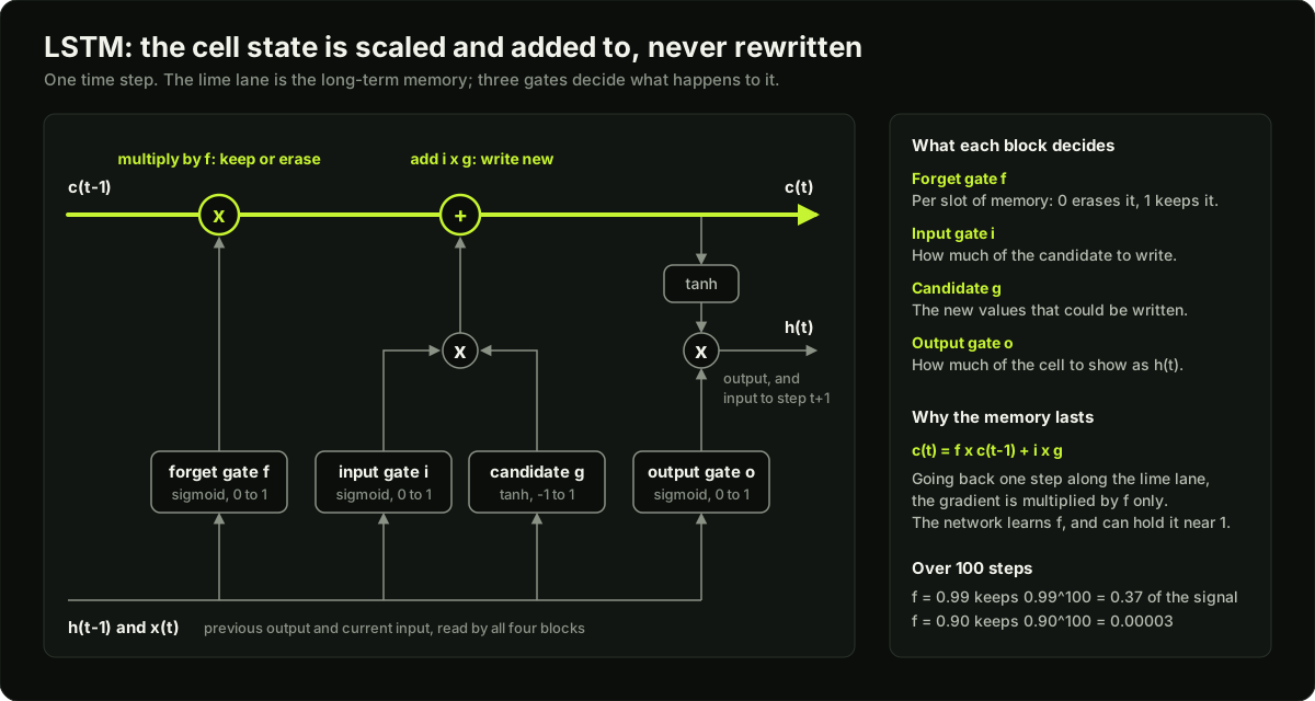 One LSTM step with the cell state as a straight lane that is multiplied by the forget gate and then added to
The forget gate f decides what to keep. The input gate i decides how much of the candidate g (new values from a tanh layer) to write. The output gate o decides how much of the cell to show as h. The important part is the first formula: the cell state is scaled and added to, and never pushed through a weight matrix. Going backward along it, the gradient is multiplied by f only, and the network can learn to hold f near 1. At f = 0.99, 0.99^100 = 0.37 survives 100 steps.
A GRU (gated recurrent unit) merges the two states and uses two gates, update and reset. It has three weight blocks where an LSTM has four, so 25% fewer parameters, with similar quality on most tasks.
Gates fix memory, not speed. An LSTM still runs step by step, and the whole past still has to fit in a fixed-size state.
CNN: one small filter, slid over the input
A convolutional neural network (CNN) slides a small filter, for example 3 x 3, over the image. At each position it takes the dot product of the filter and the patch under it. The grid of results is a feature map. A layer has many filters, each learning one pattern such as an edge or a corner.
- Few parameters. A 3 x 3 layer from 64 to 128 channels has 3 x 3 x 64 x 128 + 128 = 73,856 weights, whatever the image size.
- Position does not matter. The same filter runs everywhere, so a pattern is found wherever it appears.
- Stride and pooling shrink the map. With input size n, kernel k, padding p and stride s:
All positions in a layer are computed in parallel, which an RNN cannot do. The limit is the receptive field: the part of the input one unit can see. At stride 1, each layer of width k adds k - 1 to it, so three 3 x 3 layers see 7 x 7. Distant parts of the input meet only after many layers, and which inputs meet is fixed by the architecture, not chosen from the content.
The four designs side by side
| Model | Problem it solved | Steps for two positions n apart to interact | Parallel over positions | Limit it hit |
|---|---|---|---|---|
| RNN | Ordered input of any length | n, one after another | No | Slow training; vanishing gradients |
| LSTM, GRU | Memory over long spans | n, but the gradient survives | No | Still sequential; fixed-size state |
| CNN | Images without a weight per pixel | About n / (k - 1) layers | Yes | Fixed, local receptive field |
| Transformer | Long-range links and parallel training | 1 | Yes | Cost grows with n squared |
What survives today
- Convolutions as front-ends. A vision transformer splits a 224 x 224 image into 16 x 16 patches and applies one linear layer to each. That equals a convolution with kernel and stride 16, giving 14 x 14 = 196 tokens. Whisper, a speech recognition model, passes 3,000 spectrogram frames (30 seconds, one frame per 10 ms) through two width-3 convolutions, the second with stride 2, and hands 1,500 positions to its transformer. A convolution is a cheap way to turn a dense raw signal into a shorter sequence of tokens.
- The additive path. The LSTM cell state and the residual connection are the same idea. Every transformer block has one.
- Recurrence at inference. An LLM still generates one token at a time. The difference is what it carries forward. An RNN overwrites one fixed-size state. A transformer keeps the keys and values of every past token (the KV cache), so nothing is forgotten, and memory grows with length.
- Small recurrent models. LSTMs and GRUs are still used where memory and latency are tight, such as streaming signals on small devices.
Diagram
Worked example
One task, four designs, sized by hand. The input is a sequence of 100 tokens. Each token is a 128-number embedding, and the hidden size is 256.
- RNN parameters. One weight block reads the hidden state and the input: 256 x (256 + 128) + 256 = 98,560.
- LSTM and GRU parameters. An LSTM has four such blocks (three gates and the candidate): 4 x 98,560 = 394,240. A GRU has three: 295,680.
- Gradient from token 100 back to token 1. That is 99 steps. If a plain RNN keeps 0.9 of the gradient per step, 0.9^99 = 0.00003 is left. Along an LSTM cell state with the forget gate at 0.99, 0.99^99 = 0.37 is left. The first model cannot learn the link; the second can.
- Time. The RNN and the LSTM both need 100 steps in a row for one sequence. Making the batch larger does not shorten that chain.
- CNN. With width-3 filters at stride 1, the receptive field after L layers is 1 + 2L. To cover 100 tokens you need 1 + 2L >= 100, so 50 layers. Each layer with 256 channels in and out has 3 x 256 x 256 + 256 = 196,864 weights. Every layer runs in parallel over positions, but the two ends of the sequence only meet at layer 50.
- Self-attention. One layer links token 1 and token 100 directly. The price is one score for every pair: 100 x 100 = 10,000 per head. At 1,000 tokens that is 1,000,000, which is the quadratic cost.
Two convolution sizes worth knowing. A 7 x 7 filter with stride 2 and padding 3 on a 224-pixel side gives floor((224 + 6 - 7) / 2) + 1 = 112. A 16 x 16 filter with stride 16 and no padding gives (224 - 16) / 16 + 1 = 14 per side, so 14 x 14 = 196 patches. That second line is the patch embedding of a vision transformer.
Runnable code
"""RNN vs LSTM memory, and a CNN's receptive field, measured with NumPy.

Part 1 follows the gradient backward through time: how much of it is left
after T steps in a plain RNN, and along the cell state of an LSTM.
Part 2 stacks 1-D convolutions and finds which inputs one output can see.
"""
import numpy as np

rng = np.random.default_rng(0)
H, D = 16, 8                                   # hidden size, input size


def sigmoid(z):
    return 1 / (1 + np.exp(-z))


def rnn_gradient_left(xs, Wh, Wx):
    """Size of d h_T / d h_0: one Jacobian per step, multiplied together."""
    h, J = np.zeros(H), np.eye(H)
    for x in xs:                               # one step per token, in order
        h = np.tanh(Wh @ h + Wx @ x)           # the whole past lives in h
        J = (np.diag(1 - h ** 2) @ Wh) @ J     # tanh slope times the weight matrix
    return np.linalg.norm(J, 2)                # largest stretch factor


def lstm_gradient_left(xs, W, b):
    """Size of d c_T / d c_0 along the cell state: the product of the forget gates."""
    h, c, keep = np.zeros(H), np.zeros(H), np.ones(H)
    for x in xs:
        z = W @ np.concatenate([h, x]) + b     # all four blocks in one multiply
        f, i, o = sigmoid(z[:H]), sigmoid(z[H:2 * H]), sigmoid(z[2 * H:3 * H])
        g = np.tanh(z[3 * H:])                 # candidate values
        c = f * c + i * g                      # cell state: scale the old, add the new
        h = o * np.tanh(c)
        keep *= f                              # d c_t / d c_{t-1} on this path is just f
    return keep.mean()


def conv1d(x, kernel, stride=1):
    k = len(kernel)
    n_out = (len(x) - k) // stride + 1         # no padding
    return np.array([x[j * stride:j * stride + k] @ kernel for j in range(n_out)])


if __name__ == "__main__":
    Wh = rng.normal(0, 1 / np.sqrt(H), (H, H))
    Wx = rng.normal(0, 1 / np.sqrt(D), (H, D))
    W = rng.normal(0, 1 / np.sqrt(H + D), (4 * H, H + D))
    b = np.zeros(4 * H)
    b[:H] = 5.0                                # forget-gate bias: gates start near 1

    print("PART 1. Gradient left after T steps back through time")
    print("    T    plain RNN   LSTM cell state")
    left = {}
    for T in (1, 10, 25, 50, 100):
        xs = rng.normal(size=(T, D))
        left[T] = (rnn_gradient_left(xs, Wh, Wx), lstm_gradient_left(xs, W, b))
        print(f"  {T:3d}    {left[T][0]:.1e}     {left[T][1]:.3f}")
    assert left[100][0] < 1e-9 and left[100][1] > 0.1
    print("  the RNN factor is set by the weights and the tanh slope;")
    print("  the LSTM factor is a gate the network can learn to hold near 1")
    for f in (0.9, 0.99, 0.999):
        print(f"  a forget gate of {f} keeps {f ** 100:.1e} of the gradient after 100 steps")

    rnn_params = H * (H + D) + H
    print(f"\n  parameters with hidden {H}, input {D}: RNN {rnn_params}, "
          f"GRU {3 * rnn_params}, LSTM {4 * rnn_params}")

    print("\nPART 2. Receptive field of stacked width-3 convolutions")
    x = rng.normal(size=40)
    kernel = np.array([0.25, 0.5, 0.25])       # the same 3 weights at every position
    for layers in (1, 2, 3, 4):
        def net(v):
            for _ in range(layers):
                v = conv1d(v, kernel)
            return v
        base = net(x)
        mid = len(base) // 2                   # watch one output unit
        seen = 0
        for pos in range(len(x)):              # nudge each input in turn
            bumped = x.copy()
            bumped[pos] += 1.0
            seen += abs(net(bumped)[mid] - base[mid]) > 1e-12
        print(f"  {layers} layer(s): output length {len(base)}, one output sees {seen} inputs")
        assert seen == 1 + 2 * layers and len(base) == len(x) - 2 * layers

    strided = conv1d(conv1d(x, kernel), kernel, stride=2)
    print(f"  stride 2 in the second layer: 40 inputs -> {len(strided)} outputs")
    print("  layers needed for one output to see 1,000 inputs at stride 1:",
          int(np.ceil((1000 - 1) / 2)))
Key takeaways
RNNs and CNNs both share weights: an RNN across time steps, a CNN across positions.
A plain RNN is sequential and loses the gradient over long spans, because every step multiplies it by a weight matrix and a tanh slope.
An LSTM updates its cell state by scaling and adding, so the gradient along it is multiplied only by the forget gate, which can stay near 1. A GRU does the same job with two gates and 25% fewer parameters.
A CNN layer has kernel x kernel x channels in x channels out weights, whatever the input size, and runs in parallel over positions. Its limit is a fixed, local receptive field.
A transformer links any two positions in one step and trains in parallel, at a cost that grows with the square of the length.
Still in use: convolutions as image and audio front-ends, the additive path as the residual connection, and a recurrent loop at generation time.
Common mistakes
Saying LSTMs "solved" vanishing gradients. They protect one path, the cell state. The model is still sequential and still forgets over very long spans.
Saying gradient clipping fixes vanishing gradients. Clipping only limits exploding gradients; it cannot make a tiny gradient larger.
Saying a transformer generates in parallel. Training is parallel over positions; generation is one token at a time.
Saying modern models contain no convolutions. The patch embedding of a vision transformer and the first layers of most speech models are convolutions.
Mixing up the two LSTM states. The cell state c is the long-term memory; the hidden state h is the output of the step.
Practice
Run the code example, then set the forget-gate bias to 0 and to 2. Record the LSTM column at T = 100 for each bias and explain the change in one sentence.
By hand, compute the output size and the parameter count for three stacked layers on a 32 x 32 x 3 image: 3 x 3 filters, 16 then 32 then 64 channels, stride 2, padding 1. Check the sizes against the formula (16, 8 and 4 per side).
Explain aloud in under 90 seconds why transformers replaced RNNs and LSTMs. Record it and check that you named the sequential limit, the gradient path and the quadratic cost.
Interview questions (7)
1.Why did transformers replace RNNs and LSTMs?Easy
RNNs process tokens one by one, so they cannot be parallelised and they forget long-range context. Attention connects any two tokens directly and trains in parallel on GPUs. I would add three details. First, the path: in an RNN, information from token 1 passes through 99 updates to reach token 100, and the gradient shrinks at each one. In attention the path is one step. Second, the LSTM only half-fixed this. Its gates keep the gradient alive along the cell state, but it still runs step by step, and the whole past is squeezed into one fixed-size vector. Third, parallel training is what allowed training on far more text, and that scale is what made pretraining work. The cost is attention that grows with the square of the sequence length.
2.How does an LSTM reduce the vanishing gradient problem?Medium
A plain RNN rewrites its whole hidden state at every step by passing it through a weight matrix and a tanh. So the backward gradient is multiplied by that matrix and a slope below 1 at every step, and it fades. An LSTM adds a cell state that is updated differently: new cell equals forget gate times old cell, plus input gate times a candidate. Along that path the gradient is multiplied by the forget gate only. The gate is a learned value between 0 and 1, and the network can keep it close to 1 for information it needs. At 0.99 per step, about 37% of the gradient survives 100 steps. At 0.9 per step almost nothing does. It is the same idea as a residual connection: give the gradient an additive path.
3.LSTM vs GRU: what is the difference?Easy
Both are gated RNNs. An LSTM keeps two states, the cell state and the hidden state, and has three gates: forget, input and output. A GRU keeps one state and has two gates. The update gate decides how much of the old state to keep and how much new content to write. The reset gate decides how much of the old state is used when computing the new content. A GRU has three weight blocks where an LSTM has four, so it has 25% fewer parameters at the same hidden size and runs a little faster. Quality is similar on most tasks, so I would choose by measuring both.
4.Why do CNNs work well on images?Medium
Three properties match how images behave. First, locality: nearby pixels are related, so a small filter that looks at a 3 x 3 patch finds useful patterns such as edges. Second, weight sharing: the same filter is used at every position, so an edge detector learned in one corner works everywhere, and the layer needs few parameters. A 3 x 3 layer from 64 to 128 channels has about 74 thousand weights at any image size, while a dense layer on a 224 x 224 image needs 150 million for 1,000 units. Third, hierarchy: stacking layers with stride or pooling grows the receptive field, so early layers find edges and later layers find parts and objects.
5.What is a receptive field, and why is it a limit?Medium
It is the region of the input that can affect one unit. One 3 x 3 layer sees 3 x 3. At stride 1 each extra layer adds 2 per side, so three layers see 7 x 7. Stride and pooling make it grow faster. It is a limit for two reasons. Two things that are far apart can only be combined deep in the network, after many layers. And the wiring is fixed: a unit always reads the same neighbourhood, whatever the content is. Attention removes both: any position can read any other in one layer, and the weights are computed from the content. For text, width-3 filters at stride 1 would need about 500 layers to connect tokens 1,000 apart.
6.A transformer also generates one token at a time. How is that different from an RNN?Hard
There are two differences. In training, a transformer processes all positions of a sequence in one pass, because the causal mask lets every position predict its next token at the same time. An RNN needs one step after another even in training. At inference both loop one token at a time, but they carry different things forward. An RNN overwrites one fixed-size state, so old information is compressed and slowly lost. A transformer keeps the keys and values of every past token in the KV cache, and the new token attends to all of them directly. Nothing is forgotten inside the context window. The price is memory that grows with the sequence length, where an RNN's memory per step is constant.
7.Where are convolutions and recurrent networks still used?Easy
Convolutions are the front-end of most models that read dense signals. A vision transformer turns a 224 x 224 image into 196 patch tokens with one convolution of kernel 16 and stride 16. Speech models such as Whisper use two small convolutions to halve 3,000 spectrogram frames to 1,500 positions before the transformer. Small CNNs still run on phones and cameras because they are cheap. Recurrent models are used where memory and latency are tight, for example streaming sensor or audio signals on small devices, because their state has a fixed size. And the ideas live on: the residual connection is the LSTM's additive path, and generation is a recurrent loop.
Quiz
1.Along the LSTM cell state, what multiplies the gradient at each backward step?
2.A convolution layer has 3 x 3 filters, 16 input channels and 32 output channels. How many parameters does it have, with biases?
3.At stride 1, how large is the receptive field of one unit after four stacked 3 x 3 convolution layers?
4.Which limit do LSTMs share with plain RNNs?
5.A 224 x 224 image goes through a convolution with kernel 16, stride 16 and no padding. How many output positions are there?
Practice these problems
Further reading
My notes
Your notes
Autosaves to this browser.