What is fine-tuning - LoRA, QLoRA, DoRA
Fine-tuning changes how a model behaves by updating its weights on your examples. Updating every weight of a large model is expensive, so the LoRA family freezes the base model and trains a small add-on called an adapter, usually under 1% of the parameters. This lesson explains LoRA from the formula up, then QLoRA, DoRA and rsLoRA, and how to choose between them.
Why it matters
"Explain LoRA" is one of the most common GenAI interview questions, and the follow-ups are always the same: why does a low rank work, how do you pick rank and alpha, what does QLoRA add, does it slow inference. Each has a short, exact answer with a number in it. In real work the same knowledge decides whether a fine-tune needs one rented GPU for an afternoon or a cluster for a week, and whether you can serve fifty customer-specific models from one base model in memory.
Read first: Neural networks and backprop, LLM fundamentals - tokens, embeddings, decoding, Hugging Face end to end
Lesson
What fine-tuning changes
A pretrained model is a set of weight matrices. Fine-tuning continues training on your own examples so the weights move toward your task. Fine-tuning changes model behaviour by updating weights: output format, tone, domain vocabulary, tool-call style.
Full fine-tuning updates every weight. For a 7-billion-parameter model that means storing a gradient and optimiser state for all 7 billion values, and saving a full copy of the model for every task. PEFT (parameter-efficient fine-tuning) methods avoid this. LoRA-family methods are the most used: the base model stays frozen and you train a small adapter, usually under 1% of the parameters.
LoRA in one minute
A weight matrix W has d x k values. Instead of updating all of them, LoRA (low-rank adaptation) learns two small matrices, B (d x r) and A (r x k), and adds their product to W. The rank r is small, typically 8 to 64.
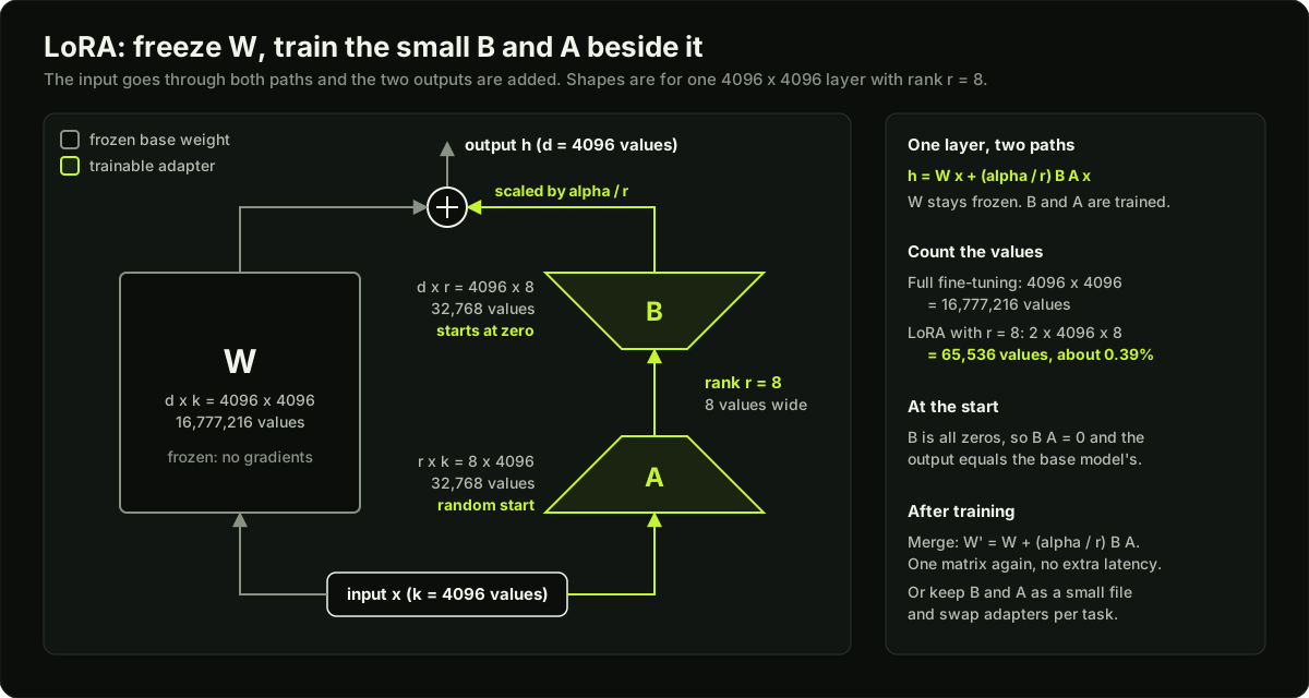 A frozen weight matrix W with a small trainable path through A and B beside it, joined by a sum
- Worked number: for a 4096 x 4096 layer, full fine-tuning updates about 16.8 million values. LoRA with r = 8 trains 2 x 4096 x 8 = 65,536 values, about 0.39%.
- Initialisation: A is random, B is zero, so the adapter starts as a zero update and training begins from the base model's behaviour.
- Alpha: a scaling factor. The update is multiplied by alpha / r. A common starting point is alpha = 2r.
- Target modules: the attention projections (query, key, value, output). Adding the MLP layers gives more capacity at more cost.
- Merge: after training you can add BA into W. The merged model has no extra latency. Kept separate, adapters are small files you can swap per customer or task.
In the forward pass the layer computes the base output and the adapter output and adds them:
A squeezes the k input values down to r values, and B expands those r values back to d. Gradients are computed only for A and B.
Why a low rank is enough
The rank of a matrix is the number of independent directions it can move its input in. A product BA with r = 8 can only change the layer's output along 8 directions, while W itself has up to 4,096.
That sounds like a harsh limit, but the pretrained model already knows the language and most of the task. Fine-tuning only has to nudge it. The LoRA paper's hypothesis is that this nudge, the change in weights during adaptation, has a low intrinsic rank: most of the useful change lives in a few directions. Two findings from that paper support it. On a model whose weight matrices were 12,288 wide, a rank of 1 or 2 was already enough for some tasks. And when the authors trained adapters with r = 8 and r = 64, the top directions the two had learned overlapped strongly, so the extra 56 directions were adding little.
The limit is real when the task is far from what the base model knows, such as a new language or a new modality. Then the needed change is not low rank, and you raise r or move to full fine-tuning.
The methods compared
| Method | What it does | Pick it when |
|---|---|---|
| Full fine-tuning | Updates every weight | You need maximum quality and have large data and many GPUs |
| LoRA | Trains low-rank matrices on a frozen base | You have GPU headroom and want fast training |
| QLoRA | LoRA on a base quantized to 4-bit (NF4) | GPU memory is the limit; fits large models on one GPU |
| DoRA | Splits each weight into magnitude and direction; LoRA updates direction, magnitude is trained separately | LoRA leaves a quality gap to full fine-tuning |
| rsLoRA | Scales by alpha / sqrt(r) instead of alpha / r | You use high ranks and training becomes unstable |
| Prompt or prefix tuning | Trains only soft prompt vectors | Many light tasks on one model; limited power |
| Adapters (classic) | Inserts small bottleneck layers | Rare now; adds inference latency because layers cannot be merged |
QLoRA is treated as the default in most open-source fine-tuning stacks in 2026, with plain LoRA chosen when memory is not the constraint.
QLoRA: three ideas that make the base 4-bit
Quantization means storing each weight in fewer bits. QLoRA loads the frozen base in 4 bits per weight and keeps the LoRA matrices in 16-bit. During the forward pass each 4-bit weight is converted back to 16-bit for the multiplication. Gradients flow through the frozen weights into A and B, and only A and B are updated. Three ideas make this work.
- NF4 (4-bit NormalFloat): 4 bits give only 16 possible values. Pretrained weights follow a bell curve centred on zero, so evenly spaced values would waste most of the 16 on the empty tails. NF4 places the 16 values so that each one covers an equal share of a normal distribution, with zero represented exactly.
- Double quantization: each block of 64 weights needs one 32-bit scale constant, which costs 32 / 64 = 0.5 extra bits per weight. QLoRA quantizes those constants too, to 8 bits. The overhead falls to about 0.127 bits per weight, a saving of about 0.37 bits. On a 65B model that is about 3 GB.
- Paged optimisers: a long sequence in a batch causes a short memory spike that would crash the run with an out-of-memory error. A paged optimiser moves optimiser state to CPU RAM during the spike and brings it back when needed.
The cost is somewhat slower training, because of the conversion on every forward pass. The QLoRA paper also found that putting LoRA on all linear layers, not only query and value, was needed to match full fine-tuning.
DoRA: magnitude and direction
Think of each column of W as an arrow. It has a length (magnitude) and a direction. LoRA's update BA changes both at once, tied together. The DoRA paper measured what full fine-tuning does and found a different pattern: it can change direction a lot while changing length only a little, or the reverse. LoRA cannot do that easily.
DoRA (weight-decomposed low-rank adaptation) separates the two:
W + BA is divided by its column lengths, so it only sets the direction. The vector m holds one trainable number per column and sets the length. m starts as the column lengths of W, so at the start W' = W, the same as LoRA. The extra parameters are tiny: one number per column. DoRA helps most at low ranks, and it can still be merged into one matrix. Training does more work per step than LoRA, and so does unmerged inference, so merge before serving.
rsLoRA: a better scaling for high ranks
With alpha fixed, LoRA's alpha / r factor shrinks the update as the rank grows. At alpha = 32, rank 16 gives a factor of 2 and rank 256 gives 0.125. The adapter learns slowly at high rank, so the extra rank buys little. Rank-stabilised LoRA (rsLoRA) divides by the square root of r, so rank 256 gives 32 / 16 = 2. The size of the update stays steady across ranks, and a higher rank can turn extra compute into quality. Nothing else changes, and inference cost is the same.
Choosing rank, alpha and target modules
Start with r = 16 and alpha = 32. Raise the rank if the task is far from what the base model knows and the eval is still improving. A higher rank means more capacity but more memory and more risk of overfitting on small data. Because the update is multiplied by alpha / r, changing alpha acts like changing the learning rate of the adapter, so tune one of them at a time. For target modules, start with the four attention projections and add the MLP layers if the eval says the adapter needs more capacity. With a 4-bit base, the QLoRA finding above makes all linear layers the usual starting point, which is what the next lesson uses.
A decision guide
- Try prompting and retrieval first. Fine-tune only when you have a stable task, a real eval and roughly 500 or more good examples.
- QLoRA is the default when the base model in 16-bit does not leave room on your GPU for training.
- LoRA when memory is not the limit: no quantization step, faster training.
- Raise the rank, with rsLoRA scaling at high ranks, if the eval is still below target.
- DoRA when LoRA at a sensible rank still leaves a gap to full fine-tuning.
- Full fine-tuning when you need the last points of quality and have large data and many GPUs.
- Prompt or prefix tuning when one model must serve many light tasks and a few trained vectors per task are enough. A soft prompt is a short list of vectors placed in front of the input and learned by gradient descent while every model weight stays frozen.
Beyond supervised fine-tuning
- SFT (supervised fine-tuning): train on input-output pairs. Always the first step.
- DPO (direct preference optimisation): train on pairs of preferred and rejected answers with one loss, no reward model. It is the usual first choice for preference tuning after SFT.
- RLHF with PPO: train a reward model on human preferences, then optimise the LLM against it. Strong but heavy to run.
- GRPO: generate a group of answers per prompt, score each with an automatic verifier (tests pass, maths correct, valid JSON), and push the model toward the above-average ones. Used for reasoning fine-tunes.
- Distillation: a large teacher model generates outputs and a small student model is trained to match them. This is how small models get close to large-model quality on a narrow task.
SFT, DPO and GRPO are commonly run on a LoRA adapter in place of the full weights, with a learning rate about 5 to 10 times higher than for full fine-tuning, because only the new parameters are being learned. The lesson on RL fine-tuning covers the last four methods in depth.
Diagram
Worked example
Counting parameters and memory for one model shape. Take a decoder with 32 layers, hidden size 4,096, MLP width 11,008 and a 32,000-token vocabulary. Each layer has four attention projections of 4096 x 4096 and three MLP matrices of 4096 x 11008.
- Base parameters. Attention: 4 x 4096 x 4096 = 67,108,864. MLP: 3 x 4096 x 11008 = 135,266,304. Per layer: 202,375,168. Times 32 layers: 6,476,005,376. Add the embedding table, 32,000 x 4096 = 131,072,000. Total: about 6.61 billion.
- LoRA on attention only, r = 16. Each projection adds 16 x (4096 + 4096) = 131,072 values. Four per layer, 32 layers: 16,777,216 values, which is 0.25% of the model.
- LoRA on attention and MLP, r = 16. Each MLP matrix adds 16 x (4096 + 11008) = 241,664 values. Per layer: 4 x 131,072 + 3 x 241,664 = 1,249,280. Times 32: 39,976,960 values, which is 0.61% of the model.
- Memory for full fine-tuning. The Adam optimiser needs the weight, its gradient and two running averages: 4 values per parameter. In 32-bit floats that is 6.61B x 16 bytes = about 106 GB before any activations.
- Memory for LoRA. The frozen base in 16-bit is 6.61B x 2 bytes = 13.2 GB. The adapter with its optimiser state is 39,976,960 x 16 bytes = 0.64 GB. Total: about 13.9 GB plus activations.
- Memory for QLoRA. The linear layers at 4.127 bits per weight (4 bits plus the double-quantized constants) take 6,476,005,376 x 4.127 / 8 = 3.34 GB. The embedding table stays in 16-bit: 0.26 GB. With the 0.64 GB adapter state: about 4.2 GB plus activations.
- What you save to disk. The adapter in 16-bit is 39,976,960 x 2 bytes = 80 MB, against 13.2 GB for a full copy of the model.
Activations and gradients through the layers add several more GB, depending on batch size and sequence length. The ordering does not change: about 106 GB, 14 GB and 4 GB for the same model.
Runnable code
"""LoRA on one linear layer with NumPy: zero start, parameter count, training, merge.

Layer convention: h = W x, with W of shape (d, k). A batch X has shape (n, k),
so the batched forward pass is H = X @ W.T.
"""
import numpy as np

rng = np.random.default_rng(0)
d, k, r, alpha = 64, 48, 4, 8          # output size, input size, rank, scaling
scale = alpha / r                      # LoRA scaling; rsLoRA would use alpha / sqrt(r)

W = rng.normal(0, 0.1, size=(d, k))    # frozen pretrained weight
A = rng.normal(0, 0.1, size=(r, k))    # trainable, random start
B = np.zeros((d, r))                   # trainable, zero start


def forward(X, W, A, B):
    """Base path plus adapter path: X W^T + scale * X A^T B^T."""
    return X @ W.T + scale * (X @ A.T) @ B.T


X = rng.normal(size=(256, k))

# 1. The adapter starts as a zero update.
print("max |B A| at start       :", np.abs(B @ A).max())
print("same output as the base  :", np.allclose(forward(X, W, A, B), X @ W.T))

# 2. Count trainable values.
full, lora = W.size, A.size + B.size
print(f"full fine-tuning values  : {full}")
print(f"LoRA values (r={r})       : {lora} = {r} x ({d} + {k}), {100 * lora / full:.1f}% of full")

# 3. Train only A and B to fit a target whose change from W has rank 2.
U, V = rng.normal(size=(d, 2)), rng.normal(size=(2, k))
Y = X @ (W + 0.05 * U @ V).T           # what the "fine-tuned" layer should output
lr = 0.01
for step in range(301):
    E = forward(X, W, A, B) - Y        # (n, d) error
    if step % 100 == 0:
        print(f"step {step:4d}  mse {np.mean(E ** 2):.6f}")
    G = E.T @ X / len(X)               # gradient w.r.t. the full update, shape (d, k)
    grad_B = scale * G @ A.T           # chain rule through delta_W = scale * B A
    grad_A = scale * B.T @ G
    B -= lr * grad_B
    A -= lr * grad_A                   # W is never touched

delta = scale * B @ A
print("rank of the learned update:", np.linalg.matrix_rank(delta), "(at most r =", r, ")")

# 4. Merge: one matrix gives the same output as base plus adapter.
W_merged = W + delta
same = np.allclose(X @ W_merged.T, forward(X, W, A, B))
print("merged == base + adapter :", same)
assert same

# 5. Unmerge by subtracting, which is how adapters are swapped on one base.
print("unmerge restores W       :", np.allclose(W_merged - delta, W))
Key takeaways
LoRA freezes W and learns W' = W + (alpha / r) BA. For a 4096 x 4096 layer at r = 8 that is 65,536 trained values, about 0.39% of the layer.
B starts at zero and A is random, so training begins exactly at the base model's behaviour.
A low rank works because the change needed to adapt a pretrained model lives in a few directions.
Start with r = 16 and alpha = 32 on the attention projections. Raise the rank only while the eval keeps improving.
QLoRA is LoRA on a 4-bit NF4 base, with double quantization and paged optimisers. It is the default when GPU memory is the limit.
DoRA trains magnitude separately and applies LoRA to direction. rsLoRA scales by alpha / sqrt(r) for high ranks.
Merged adapters add no latency. Unmerged adapters let one base model serve many tasks or customers.
Common mistakes
Saying LoRA "trains a smaller model". The base model still runs in full on every forward pass; only the trained part is small.
Initialising both A and B to zero. Each one's gradient depends on the other, so nothing ever updates.
Changing rank and alpha together and then not knowing which one helped. The effective scale is alpha / r.
Raising the rank to fix a problem that is really bad data or a wrong chat template.
Assuming QLoRA makes inference cheaper. It lowers training memory; serving cost depends on how you load the base at inference time.
Quoting the adapter size as the training memory. The frozen base and the activations still have to fit on the GPU.
Practice
Implement a LoRA linear layer in NumPy or PyTorch with forward, merge and unmerge. Assert that the merged output matches base plus adapter to 1e-6.
For a model you can load, count the parameters LoRA adds at r = 8, 16 and 64 on the attention projections only, then on all linear layers. Report each as a percentage of the base.
Train the same adapter with r = 4, 16 and 64 on 1,000 examples and plot validation loss. Report the rank at which the eval stops improving.
Load one model in 16-bit and in 4-bit and record peak GPU memory for a single training step with the same batch.
Interview questions (13)
1.Explain LoRA. Why does a low rank work?Medium
LoRA freezes the base weights and learns a low-rank update BA. For a d x k matrix, B is d x r and A is r x k, and the layer computes W x plus alpha over r times B A x. It works because the change needed to adapt a pretrained model to a task has low intrinsic rank: most of the useful change lives in a few directions, so a small matrix pair captures it. The base model already knows the language; the adapter only nudges it. For a 4096 x 4096 layer, r = 8 trains 65,536 values, not 16.8 million, about 0.39%.
2.How do you choose rank and alpha?Medium
Start with r = 16 and alpha = 32. Raise the rank if the task is far from what the base model knows and the eval is still improving. A higher rank means more capacity but more memory and more risk of overfitting on small data. Alpha over r multiplies the update, so alpha behaves like a learning-rate multiplier for the adapter; I keep alpha at twice the rank and tune the learning rate. If I go to high ranks I switch to rsLoRA scaling, alpha over the square root of r, so the update does not shrink.
3.LoRA vs QLoRA?Medium
Both learn the same low-rank update. QLoRA also loads the frozen base in 4-bit, which cuts memory enough to fine-tune a 70B-class model on one 80 GB GPU. It adds three things: NF4 quantization, double quantization, and paged optimizers. The cost is somewhat slower training, because the 4-bit weights are converted to 16-bit on every forward pass. I use QLoRA when memory is the limit and plain LoRA when the model fits comfortably.
4.What does DoRA fix?Hard
LoRA changes the magnitude and direction of weights together, which differs from how full fine-tuning behaves. DoRA separates them and applies the low-rank update to direction only, with the magnitude as a small trainable vector, one number per column. It usually closes part of the gap to full fine-tuning, most clearly at low ranks, and it can still be merged, so inference cost is unchanged. The price is more compute per training step, and unmerged inference is slower than plain LoRA, so I merge before serving.
5.Does LoRA slow down inference?Easy
Not if you merge it. Merging adds alpha over r times BA into W, so the layer is one matrix again with the same shape and the same latency as the base model. Unmerged adapters add a small cost, because each adapted layer does two extra small matrix multiplications, but they let one base model serve many adapters at once (multi-LoRA serving). That is how you serve one fine-tune per customer without one GPU per customer.
6.How much data do you need?Easy
For tone or instruction following, 500 to 2,000 clean examples often beat tens of thousands of noisy ones. Domain adaptation needs more, around 5,000 to 20,000. Preference tuning with DPO needs about 1,000 to 5,000 pairs. Quality and match to real inputs matter more than volume, so I would rather spend a day cleaning 1,000 examples than add 10,000 unchecked ones.
7.What is catastrophic forgetting?Medium
The model gets better at the new task and worse at things it knew before. Reduce it with PEFT instead of full fine-tuning, a lower learning rate, fewer epochs, mixing in general data, and a regression eval on general tasks. With LoRA the base weights are frozen, so the damage is limited to what the adapter adds, and removing the adapter gives the original model back.
8.RLHF vs DPO vs GRPO?Hard
RLHF needs a reward model and online sampling: you train a model to score answers from human preferences, then optimise the LLM against it with PPO. DPO needs only preference pairs and one training pass, with no reward model. GRPO needs a verifier that can check answers automatically, not human labels: it samples a group of answers per prompt and pushes the model toward the above-average ones. Choose by what signal you have: pairs of better and worse answers mean DPO, an automatic checker means GRPO.
9.How do you evaluate a fine-tuned model before shipping?Medium
Hold out 10 to 20% of the data. Score the base and the fine-tuned model on the same prompts with task metrics and an LLM judge. Then run a regression check on general tasks to catch forgetting. If the gain is not clear, do not ship. I also compare against the base model with its best prompt, not a weak prompt, so the fine-tune has to beat the real alternative.
10.Your fine-tuned model is worse than the base. What went wrong?Hard
Common causes: wrong chat template or missing special tokens, learning rate too high, too many epochs on small data, noisy or mislabelled examples, or training data that does not match production inputs. Check the template first; it is the most frequent bug. I print one fully formatted training example and one inference prompt as raw text and compare them token by token before looking at anything else.
11.Why is B initialised to zero and A to random values? What if both were zero?Hard
With B at zero the product BA is zero, so the first forward pass is exactly the base model and training starts from known-good behaviour. A must not be zero as well. The gradient for B is the layer gradient times A transposed, and the gradient for A is B transposed times the layer gradient. If both are zero, both gradients are zero and nothing ever moves. With A random and B zero, B gets a gradient on step one, and A starts moving as soon as B is non-zero.
12.What do NF4, double quantization and paged optimisers do in QLoRA?Hard
NF4 is a 4-bit data type built for weights that follow a bell curve. It places its 16 values so each covers an equal share of a normal distribution, which keeps more information than evenly spaced values. Double quantization compresses the per-block scale constants themselves, from 32-bit to 8-bit, saving about 0.37 bits per weight, around 3 GB on a 65B model. Paged optimisers move optimiser state to CPU memory during short spikes, such as a batch with a very long sequence, so the run does not die with an out-of-memory error.
13.Where does GPU memory go during fine-tuning, and what does LoRA actually save?Hard
Four places: the weights, their gradients, the optimiser state, and the activations kept for backpropagation. Adam keeps two extra values per trained parameter, so full fine-tuning needs about four values per weight. LoRA removes the gradient and optimiser state for the frozen weights, which is most of it. It does not remove the base weights or the activations, because the full model still runs forward and gradients still flow back through every layer. QLoRA then shrinks the base weights about four times by storing them in 4 bits.
Quiz
1.A layer has a 2048 x 2048 weight matrix. How many values does LoRA with r = 16 train for it?
2.Right after initialisation, how does a LoRA model's output compare with the base model's?
3.Which statement about QLoRA is correct?
4.With alpha = 32, what is the scaling factor for r = 64 under LoRA and under rsLoRA?
5.You must serve 40 customer-specific fine-tunes of one base model on a single GPU. What is the best fit?
Practice these problems
Further reading
My notes
Your notes
Autosaves to this browser.