Finetuning adapts a pretrained model by continuing to train some or all of its weights on your own data. It is the heaviest tool in the application developer's kit: it can teach a model a format, a style or a domain's habits that no prompt reliably produces, and it can make a small, cheap model good enough to replace an expensive one. It also costs data, GPUs, ML expertise and an ongoing maintenance commitment, and it can quietly make a model worse at everything you did not finetune for.

This chapter is about making that call well and executing it cheaply. It covers when finetuning is the right lever (and when retrieval or a better prompt is), why training a model needs several times the memory of serving it, how low-precision formats and quantization shrink that bill, how parameter-efficient methods such as LoRA get most of the benefit for a fraction of the cost, how finetuned models can be merged without any training at all, and which hyperparameters actually matter. The running theme is memory: almost every technique in the chapter exists to do more adaptation with fewer bytes.

In one minute

• Finetuning is transfer learning on a foundation model. It changes behaviour (format, style, domain conventions, consistency); RAG changes knowledge. Diagnose the failure before choosing the fix: information-based failures want retrieval, behaviour-based failures want finetuning.
• Try prompt engineering and few-shot examples first, then RAG, then finetuning. Many production applications never need to finetune; those that do usually also keep RAG.
• Training memory is dominated by things that do not exist at inference: gradients, optimizer states and saved activations. For full finetuning with Adam, budget roughly 8 bytes per parameter in pure BF16 and about 16 bytes per parameter with standard mixed precision, before activations.
• Numerical formats trade range (exponent bits) against precision (mantissa bits). BF16 keeps FP32's range in half the bytes and is the default for LLM training; INT8 and INT4 are mostly inference formats.
• Quantization is cheap to apply at inference (post-training, weight-only) and hard during training; QLoRA threads the needle by quantizing the frozen base to 4 bits while training BF16 adapters.
• Parameter-efficient finetuning (PEFT) trains a small set of new parameters. LoRA, which learns a low-rank update W + BA, dominates in practice because it adds no inference latency once merged and lets many adapters share one base model.
• Model merging combines finetuned checkpoints without gradients: summing task vectors (with TIES or DARE to cut interference), stacking layers (franken-merging, depth upscaling, MoE upcycling) or concatenating adapters.
• Tactics that matter: pick the base model with the development path in mind (progression vs distillation), start from a framework's defaults, and watch learning rate, batch size, epochs and prompt loss weight. Data quality beats hyperparameter search.

Finetuning overview

What finetuning is

Finetuning is transfer learning: knowledge a model acquired on one task (predicting the next token over a web-scale corpus) is reused to learn a second task from far less data than training from scratch would need. Pretraining is the expensive, general phase; finetuning is the cheap, specific phase. The same mechanism underlies the post-training that model providers do (supervised finetuning and preference finetuning turn a raw language model into a chat assistant), the domain adaptation that teams do on top (continued pretraining on medical or legal text), and the task-specific finetuning that application developers do (teach the model your JSON schema, your tone, your product catalogue's conventions).

There are two ways to transfer. Feature-based transfer freezes the pretrained model and uses its outputs (embeddings, hidden states) as fixed features for a separate, small model trained on top; classic word2vec pipelines and most embedding-plus-classifier setups work this way. Finetuning-based transfer continues to update the pretrained weights themselves, so the internal representations can reshape around the new task. Everything in this chapter is finetuning-based transfer, including the parameter-efficient methods that only update a sliver of the network: they still change what the model computes, not just what you do with its outputs.

Two features of modern foundation models make finetuning unusually effective. First, sample efficiency: a model that already knows language and the world needs a few hundred to a few thousand examples to pick up a new format or domain, where a model trained from scratch would need millions. Second, the better the base model, the less finetuning it needs and the fewer parameters have to move. That second point is why small adapters work at all, and why the chapter spends so much time on them.

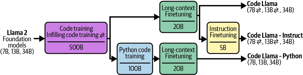How the Code Llama family was made from Llama 2 with code training, Python training, long-context finetuning and instruction finetuning

Finetuning is also layered in practice. Code Llama was not one finetuning run but a tree: Llama 2 was continued-pretrained on code, then branched into a Python specialist, a long-context variant and an instruction-following variant. Each branch is a finetuning run on the previous checkpoint, and each stage used data chosen for that stage's goal. Application teams rarely go this far, but the pattern matters: the model you finetune is itself the product of several finetuning steps, and your run is one more branch on that tree.

Prompting versus finetuning

Prompting and finetuning solve overlapping problems with different mechanisms. A prompt puts instructions and examples in the model's input while the weights stay frozen; the model has to rediscover what you want on every request, and you pay for those tokens every time. Finetuning moves that information into the weights: the behaviour is there without being asked for, the prompt gets shorter and cheaper, and the behaviour tends to be more consistent because it does not depend on the model reading and obeying a long instruction block.

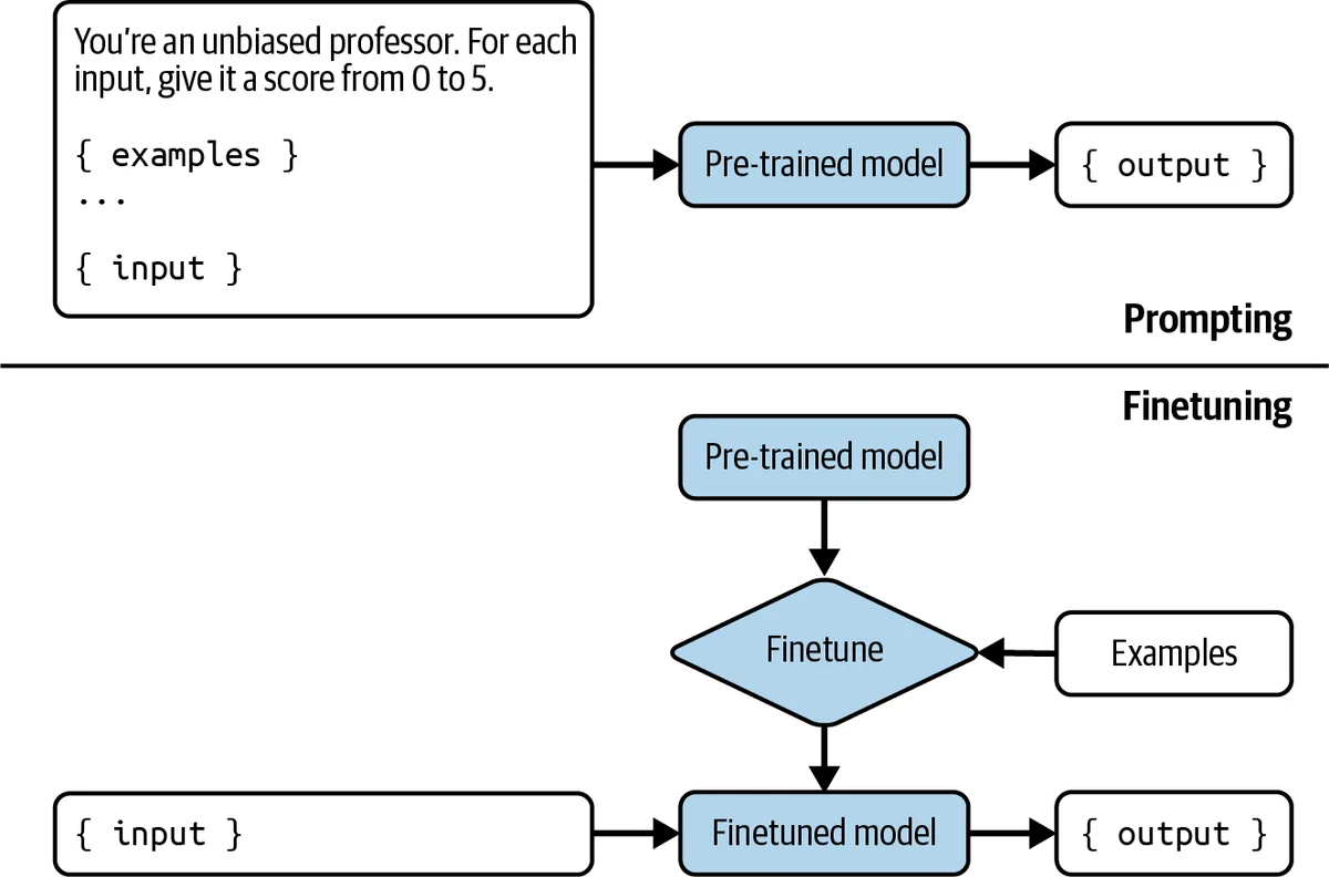Prompting puts examples in the input of a frozen model; finetuning changes the model's weights

The costs sit on the other side of the ledger. A prompt change ships in minutes and can be tested with a handful of examples; a finetuning run needs curated data, GPUs, an evaluation harness and a release process. A prompt can be inspected; a weight change cannot. When the base model is upgraded, your prompt probably still works, while your finetuned checkpoint has to be retrained. Treat finetuning as a product investment with an upkeep schedule, not as a one-off fix.

Reasons to finetune

The book's case for finetuning rests on a few concrete wins rather than vague "better performance" claims.

Task-specific quality. On a narrow task with a clear target, a finetuned model usually beats a prompted general model of the same size, and a finetuned small model can beat a prompted large one. The gains are largest where the task has conventions the model has to learn rather than facts it has to know: domain vocabulary, house style, how your product refers to things, how to decompose a particular kind of request.

Structured outputs and format adherence. Models prompted to emit strict JSON, YAML, SQL dialects or a custom DSL fail a small but costly fraction of the time. Finetuning on a few hundred correctly formatted examples drives that failure rate down far more reliably than ever-longer format instructions, and it does so without spending prompt tokens on the schema on every call.

Consistency and bias correction. Finetuning can push a model toward stable behaviour across paraphrases of the same request, and it can counteract systematic biases in the base model (for example, a tendency to associate professions with a gender) by training on examples that exhibit the behaviour you want.

Making a small model good enough. The commercially strongest reason is cost and latency. A 7B or 13B model finetuned on outputs from a frontier model (distillation, covered in the data chapter) often matches the frontier model on a specific task at a tenth of the inference cost, runs on hardware you control, and returns tokens faster. If you are making millions of calls a day, this is where finetuning pays for itself.

Data residency. When data cannot leave your infrastructure, an open-weight model finetuned on-premises may be the only option that reaches acceptable quality.

Reasons not to finetune

Finetuning is also the step most teams reach for too early. The book is explicit that many applications never need it, and it lists what goes wrong when they try.

It can degrade everything you did not train for. A model finetuned on one task frequently gets worse at adjacent tasks, and sometimes at instruction following in general. This is catastrophic forgetting in a mild form: the weight updates that encode the new behaviour overwrite representations that other behaviours depended on. You now need an evaluation suite that covers the capabilities you still care about, not just the one you targeted.

It is bad at teaching facts. Finetuning on new knowledge is unreliable and, according to work such as Gekhman et al. (2024), can increase hallucination: the model learns to produce confident answers in the new domain faster than it learns the facts, and generalizes that confidence to things it was never told. Knowledge that changes, or that must be cited, belongs in retrieval.

It needs data you may not have. Supervised finetuning wants hundreds to tens of thousands of high-quality input/output pairs that look like production traffic. Collecting, cleaning and annotating them is usually the most expensive part of the project; the training run itself is a few hours of GPU time.

It needs ML skills and infrastructure. Someone has to choose a base model and method, set hyperparameters, read loss curves, debug out-of-memory errors, version checkpoints and evaluate the result. Managed finetuning APIs remove some of this but not the data or evaluation work.

It creates a maintenance liability. Base models improve every few months. Each time a new one is clearly better than yours, you either repeat the pipeline or fall behind. Prompt-based and retrieval-based systems inherit upgrades for free.

The ceiling may be lower than you think. Studies comparing prompting, RAG and finetuning repeatedly find that for knowledge-heavy tasks RAG wins and for many behaviour tasks a carefully engineered prompt gets most of the way. Measure the gap with a strong prompt before paying to close it.

Finetuning and RAG: context versus behaviour

The most useful framing in the chapter is a diagnostic. When a model fails, ask whether it failed because it lacked information or because it behaved badly with the information it had.

Failure looks like	Root cause	Fix
Wrong, outdated or made-up facts; "I don't know your product"	Missing or stale information	RAG (give the model the context)
Right facts, wrong format; ignores schema; inconsistent tone	Behaviour the model has not learned	Finetuning
Correct in isolation but mis-uses retrieved documents (ignores them, cites the wrong one)	Behaviour on top of context	Finetune on examples that include retrieved context
Too slow or too expensive at acceptable quality	Model too large for the task	Finetune a smaller model (distillation)
Fails only on long-tail inputs	Coverage gap in prompt examples or data	More examples in the prompt, then more finetuning data

The two techniques are complementary rather than rivals. RAG supplies what the model should know for this request; finetuning shapes how the model uses what it is given. Teams that do both typically finetune on examples whose inputs already contain retrieved passages, so the model learns to read, weigh and cite context in the exact shape the production pipeline produces. Finetuning on bare questions and then bolting retrieval on afterwards trains the model for a distribution it will never see.

Two experimental results anchor the framing. Ovadia et al. (2023) compared finetuning with RAG for injecting knowledge and found retrieval consistently more effective, with finetuning only helping when combined with retrieval. The Gekhman et al. result above explains why: finetuning moves the model's willingness to answer faster than its knowledge.

The development path

The book's recommended order of operations keeps the expensive steps last and makes each step informative for the next.

1. Prompt engineering first. Write a careful system prompt, add explicit output format instructions, and build an evaluation set while you do it. The evaluation set is the real deliverable: without it you cannot tell whether any later step helped.
2. Add examples. Few-shot examples in the prompt fix many format and style problems. If the model needs twenty examples to behave, that is also a signal that finetuning would work, because you have shown it is learnable from examples.
3. Add retrieval when failures are about information. Most "the model doesn't know X" problems end here.
4. Finetune when the remaining failures are about behaviour: format, consistency, domain habits, or when the only model that behaves well is too expensive.
5. Combine. Production systems that finetune almost always keep retrieval, and often finetune on inputs that contain retrieved context so the two are trained together.
6. Shrink. Once a large model does the task well, its outputs become training data for a smaller model. This distillation path is how many teams get frontier quality at small-model prices.

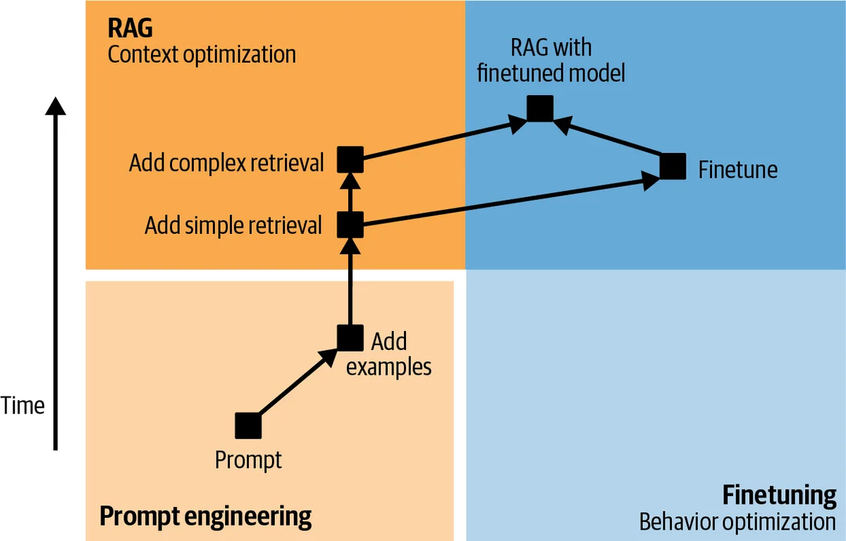A typical application development path: prompt engineering first, then retrieval for context, then finetuning for behaviour, and often both together

The path is not strictly linear. Some teams start by finetuning a small model if they already have plenty of labelled data and tight latency requirements. But every detour should be justified against the evaluation set built in step one.

Memory bottlenecks

Finetuning is expensive because training a model needs far more memory than running it. Knowing exactly where that memory goes explains why PEFT, quantization and QLoRA work, and lets you estimate hardware needs before you start.

Backpropagation and trainable parameters

A training step has two passes. The forward pass computes the model's output from the input, exactly as inference does, but it also stores the intermediate results (activations) of every layer. The backward pass uses those activations and the loss to compute a gradient for every trainable parameter, propagating error from the output back to the input through the chain rule. The optimizer then updates each trainable parameter using its gradient and, for adaptive optimizers such as Adam, running statistics of past gradients called optimizer states.

The key word is trainable. Gradients and optimizer states are needed only for parameters that will be updated. Frozen parameters still take part in the forward and backward passes (their activations must be stored and gradients must flow through them), but they need no gradient storage of their own and no optimizer state. This is the single fact that makes parameter-efficient finetuning cheap: freezing 99% of the model removes 99% of the gradient and optimizer memory.

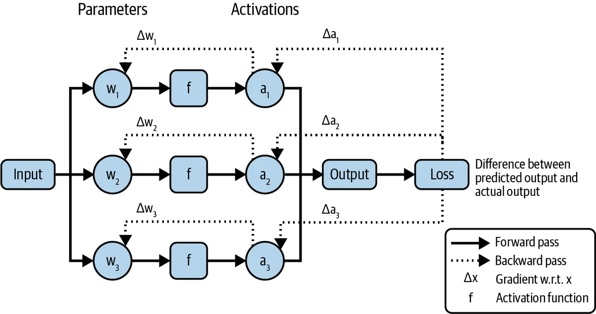Memory during training: parameters, activations from the forward pass, and gradients from the backward pass all have to fit

Memory math

For inference, memory is approximately the weights plus a modest overhead for activations and the KV cache. The book's rule of thumb is to budget about 20% on top of the weights: a 13B-parameter model in BF16 (2 bytes per parameter) needs 26 GB for weights and roughly 31 GB in total. (Long contexts and large batches push the KV cache well past that 20%; the inference chapter does that calculation properly.)

For training with all parameters trainable, each parameter carries several values.

Component	Values per trainable parameter	Pure BF16 (bytes)	Standard mixed precision (bytes)
Weights	1	2	2 (BF16 working copy) + 4 (FP32 master copy)
Gradients	1	2	2
Adam optimizer states	2 (first and second moment)	4	8 (kept in FP32)
Total before activations		8	16

With the simpler accounting the book uses, a 13B model needs 13 × 10⁹ × 8 bytes ≈ 104 GB before activations, already more than an 80 GB GPU. With the mixed-precision recipe that most frameworks actually use (the "16 bytes per parameter" from the ZeRO paper), it is about 208 GB. Either way, full finetuning of a 13B model does not fit on one GPU, and a 70B model needs a multi-node cluster.

Activations add a term that scales with batch size × sequence length × hidden size × number of layers, plus attention score matrices that scale with the square of the sequence length unless a fused attention kernel avoids materializing them. For large models and long sequences, activations, not weights, dominate training memory. Activation recomputation (also called gradient checkpointing) stores only a subset of activations and recomputes the rest during the backward pass, trading roughly a third more compute for a large memory reduction; it is on by default in most finetuning frameworks.

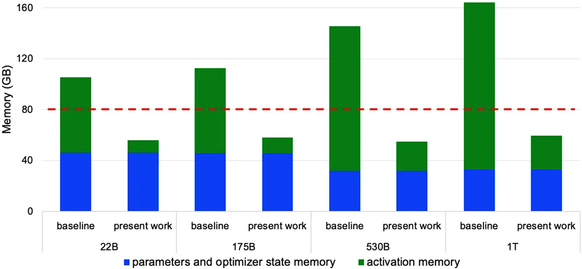Activation memory dominates training memory at scale, which is why activation recomputation matters

Put the pieces together and you get the three levers every memory-saving technique pulls:

1. Fewer trainable parameters (PEFT) removes gradients and optimizer states for the frozen majority.
2. Fewer bytes per value (lower precision, quantization) shrinks weights, and sometimes gradients and states.
3. Fewer stored activations (recomputation, shorter sequences, smaller micro-batches with gradient accumulation).

Numerical representations

A floating-point number spends its bits on a sign, an exponent (which sets the range of magnitudes it can represent) and a mantissa or significand (which sets the precision within that range). Formats differ in how they split a fixed budget.

Format	Total bits	Exponent	Mantissa	Range	Typical role
FP32	32	8	23	~3.4 × 10³⁸	Master weights, optimizer states, accumulation
TF32	19 used (stored in 32)	8	10	~3.4 × 10³⁸	Tensor-core matmul input on Ampere and later
FP16	16	5	10	~65,504	Mixed precision with loss scaling; inference
BF16	16	8	7	~3.4 × 10³⁸	Default for LLM training and serving
FP8 E4M3	8	4	3	~448	Weights and activations on Hopper and later
FP8 E5M2	8	5	2	~57,344	Gradients (needs range more than precision)
INT8	8	–	–	−128 to 127	Post-training inference quantization
INT4 / NF4	4	–	–	16 levels	Weight-only inference quantization; QLoRA base

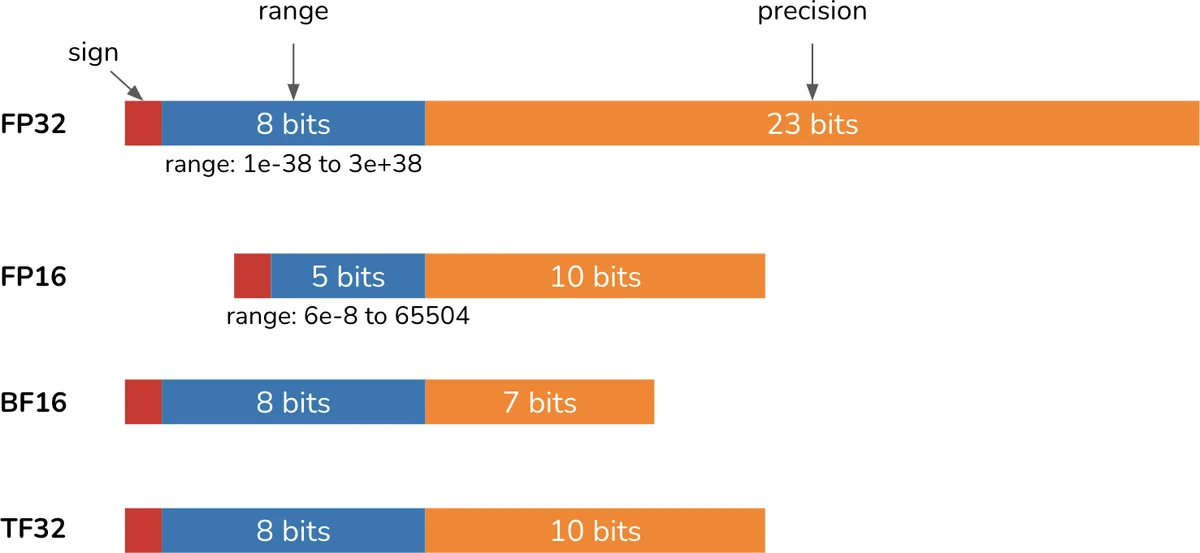Floating point formats compared: how many bits each spends on exponent (range) and mantissa (precision)

Two consequences follow from the table. FP16 overflows and underflows easily: its maximum is 65,504, and gradients during training routinely leave that range, which is why FP16 mixed precision needs loss scaling to keep small gradients from flushing to zero. BF16 was designed to avoid this by keeping FP32's 8 exponent bits and giving up mantissa bits instead; neural network training tolerates imprecision far better than it tolerates overflow, so BF16 has become the default for LLMs. TF32 is a hardware trick rather than a storage format: Ampere tensor cores read FP32 inputs, round them to 10 mantissa bits internally, and run the multiply at near-FP16 speed while accumulating in FP32.

Mixed precision training (Micikevicius et al., 2017) keeps an FP32 master copy of the weights and does the forward and backward computation in FP16 or BF16, which is where the 16-bytes-per-parameter figure comes from. Lower precision speeds up both training and inference because modern accelerators deliver several times more FLOP/s at 16 bits than at 32, and far more again at 8 bits.

Quantization

Quantization maps values from a higher-precision format to a lower-precision one, usually from 16-bit floats to 8-bit or 4-bit integers, by choosing a scale (and often a zero point) per tensor, per channel or per small block, then rounding. The goal is fewer bytes and faster arithmetic at an acceptable loss of fidelity. Two questions organize the design space: what gets quantized and when.

What. Weights are the obvious target because they are the bulk of a model's memory and their distribution is well behaved. Activations can also be quantized, which is required to actually run the matmuls in low-precision arithmetic rather than dequantizing weights on the fly; but activations in large transformers contain outlier features, a few channels with values orders of magnitude larger than the rest. A single per-tensor scale wastes almost all its resolution on those outliers and crushes everything else to zero. LLM.int8() (Dettmers et al., 2022) handles this with a mixed decomposition that keeps outlier channels in 16-bit; SmoothQuant migrates the difficulty from activations into weights with a per-channel rescaling; GPTQ and AWQ pick weight rounding that minimizes output error on calibration data. The KV cache is a third target with its own quantization tricks.

When: inference quantization. Post-training quantization (PTQ) quantizes an already-trained model, typically weight-only to INT8 or INT4, using a small calibration set or none at all. It is cheap, widely supported (GGUF, GPTQ, AWQ, bitsandbytes) and the first optimization most serving stacks apply. Quality loss is usually small at 8 bits and noticeable but often acceptable at 4 bits; it grows as models get smaller, because small models have less redundancy to absorb rounding error.

When: training quantization. Training in low precision is much harder, because gradient updates are small and rounding them away stalls learning. The practical options are mixed precision (compute in BF16, accumulate and store masters in FP32), FP8 training on hardware that supports it (with careful per-tensor scaling), and quantization-aware training (QAT), which simulates the quantization noise during training so the model learns to tolerate it. Research pushes further: BitNet b1.58 trains models whose weights take only the values {−1, 0, 1}. These are frontier-lab techniques; application teams encounter training quantization almost exclusively through QLoRA.

QLoRA (Dettmers et al., 2023) is the bridge. The frozen base model is stored in 4-bit NormalFloat (NF4), a data type whose 16 levels are placed at the quantiles of a normal distribution, which is a good match for weight distributions. Those weights are dequantized to BF16 on the fly for each matmul, and gradients flow through them to small BF16 LoRA adapters that are the only trainable parameters. Double quantization quantizes the per-block scale factors themselves, saving about 0.4 bits per parameter. Paged optimizers spill optimizer states to CPU memory via unified memory when a long sequence causes a spike. The result was finetuning a 65B model on a single 48 GB GPU, with the Guanaco models reaching about 99% of ChatGPT's score on the Vicuna benchmark as judged by GPT-4. The lesson generalizes: quantize the parts that do not move, keep the parts that move in a format that can represent small updates.

Finetuning techniques

Partial finetuning and the case for PEFT

The cheapest way to reduce training memory is to freeze most of the network and update only some layers, usually the top ones. This partial finetuning cuts gradient and optimizer memory in proportion to what is frozen, but Houlsby et al. (2019) showed that it is parameter-inefficient: to approach full-finetuning quality on GLUE you had to unfreeze about a quarter of BERT. Their alternative, inserting small adapter modules into every layer and training only those, matched full finetuning to within a fraction of a point while adding roughly 3.6% new parameters per task. That gap, far fewer trainable parameters for the same quality, is what defines parameter-efficient finetuning (PEFT).

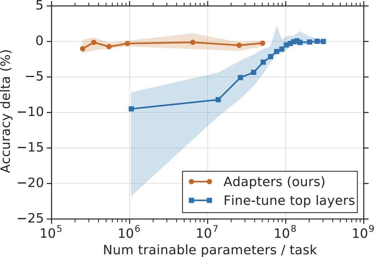Adapters match full finetuning of the top layers with orders of magnitude fewer trainable parameters per task

PEFT methods share a motivation (maximum adaptation per byte of trainable state) and split into two families by where the new parameters live.

Family	Idea	Representative methods	Inference overhead
Adapter-based (additive)	Add new trainable modules or matrices alongside frozen weights	Houlsby adapters, LoRA and variants, IA³, LongLoRA	Adapters: extra sequential compute; LoRA: zero once merged
Soft-prompt-based	Add trainable continuous vectors to the input or to each layer's attention inputs, leave weights untouched	Prompt tuning, prefix tuning, P-tuning	A few extra tokens of context per request

A third, less common family, selective methods such as BitFit (train only bias terms), updates a sparse subset of existing weights rather than adding any; the book treats it as a footnote and so does practice.

Adapter-based methods

An adapter in the Houlsby sense is a bottleneck block: a down-projection from the hidden size d to a small bottleneck m, a nonlinearity, an up-projection back to d, and a skip connection so the block starts out close to the identity. Two adapters go into each transformer layer (after attention and after the feed-forward block), and only they are trained. With m around 64 against d of several thousand, the parameter count is small.

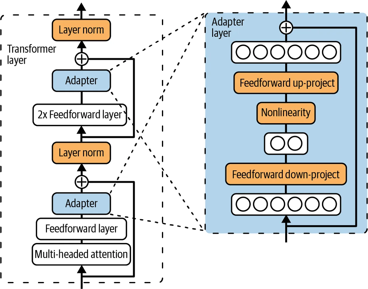Adapter modules inserted into a transformer layer: a down-projection, a nonlinearity and an up-projection with a skip connection

The drawback is that adapters sit in the forward path: every request pays for the extra sequential compute, which matters for latency-sensitive serving. LoRA, discussed next, is also adapter-based but places its new parameters in parallel with an existing weight matrix, so they can be folded back into that matrix after training and cost nothing at inference. That difference is most of why LoRA replaced classic adapters.

LoRA in detail

Low-Rank Adaptation (Hu et al., 2021) freezes a pretrained weight matrix W (shape d × k) and learns an update ΔW as the product of two small matrices: B (d × r) and A (r × k), with rank r much smaller than d and k. The layer computes h = Wx + (α / r) · BAx. A is initialized randomly and B to zero, so BA is zero at the start and the model begins exactly where the pretrained model left off. Only A and B get gradients and optimizer states; W never changes.

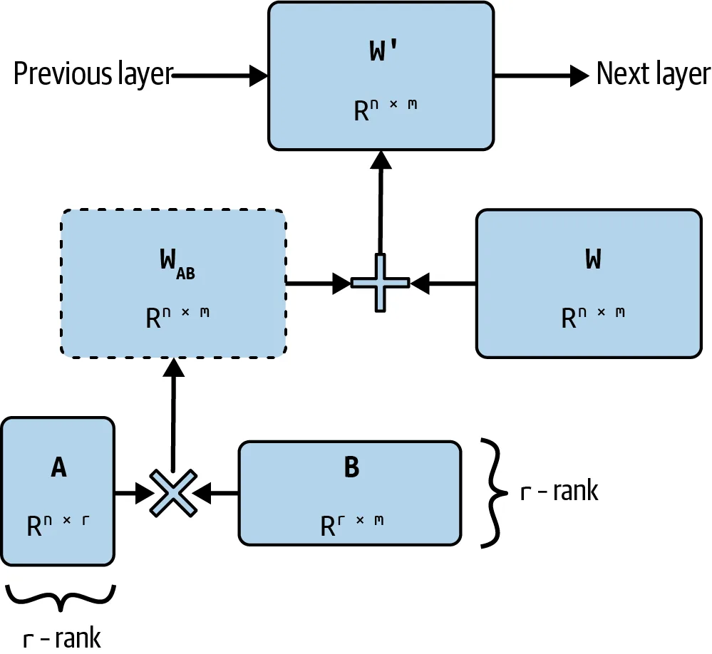LoRA: the update to a weight matrix W is factored into two small matrices A and B of rank r

A full update has d × k parameters; the LoRA update has r × (d + k). For a 4096 × 4096 projection and r = 16 that is 16.8 million versus 131 thousand, a reduction of about 128×. Across a whole model the original paper reported a 10,000× reduction in trainable parameters and a 3× reduction in GPU memory for GPT-3 175B with no loss in quality on its benchmarks.

Why low rank is enough. Aghajanyan et al. (2020) showed that pretrained language models have a low intrinsic dimension: the finetuning solution for a task lives in a subspace with far fewer dimensions than the parameter count, and the larger and better-trained the model, the lower that dimension. LoRA is a direct bet on this: constrain the update to a low-rank subspace and you lose little. The bet has limits worth stating in interviews. It holds for finetuning, not pretraining (where updates need full rank, hence approaches such as GaLore). And on tasks far from the pretraining distribution, such as heavy code or maths training, "LoRA Learns Less and Forgets Less" (Biderman et al., 2024) found full finetuning still ahead on the target task, with LoRA's compensation being that it damages other capabilities less.

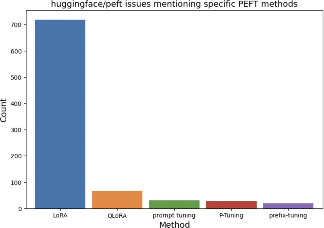Issues in the huggingface/peft repository that mention each method: LoRA dominates

Which matrices. A transformer layer has four attention projections (query Wq, key Wk, value Wv, output Wo) and two or three feed-forward matrices. The LoRA paper, holding the trainable budget fixed at about 18M parameters on GPT-3, compared where to spend it.

Matrices adapted	Rank r	WikiSQL accuracy	MultiNLI accuracy
Wq only	8	70.4	91.0
Wk only	8	70.0	90.8
Wv only	8	73.0	91.0
Wo only	8	73.2	91.3
Wq and Wk	4	71.4	91.3
Wq and Wv	4	73.7	91.3
Wq, Wk, Wv, Wo	2	73.7	91.7

Spreading a fixed budget across more matrices at lower rank beat concentrating it in one matrix at higher rank. Later practice went further: most frameworks now default to applying LoRA to every linear layer, including the feed-forward projections, because the feed-forward blocks hold most of a modern model's parameters and much of its task-specific knowledge.

Rank and alpha. The rank r controls capacity. The paper found ranks of 1 to 4 competitive with 64 on its tasks; practitioners typically start at 8 or 16 and go to 64 or 128 only for hard domain shifts. The scaling factor α sets how strongly the update is applied relative to the base weights; because the update is multiplied by α / r, raising r at fixed α shrinks each component's contribution. Common heuristics set α equal to r or to 2r, then tune the learning rate rather than α. A variant, rsLoRA, scales by α / √r so that larger ranks do not learn more slowly.

Adapter size. The memory story at inference is what makes LoRA operationally attractive. With r = 16 on the four attention projections in BF16, a Llama 2 7B adapter is about 34 MB against 13.5 GB of base weights; 13B gives about 52 MB; 70B (with grouped-query attention shrinking Wk and Wv) about 130 MB; GPT-3 175B about 300 MB. Hundreds of task adapters fit in the memory one extra base model would need.

Serving LoRA: merging and multi-LoRA

After training there are two ways to serve.

Merge. Compute W' = W + (α / r) · BA once and save W' as an ordinary dense checkpoint. Inference is identical to the base model: no extra kernels, no latency. The cost is a full model copy per task, and a merged model cannot be "un-merged" if you later want to swap adapters.

Keep separate. Load the base once and apply adapters at request time. A serving engine can hold many adapters in memory, batch requests for different adapters together (because the expensive base matmul is shared and only the small BA matmuls differ per request), and swap adapters in and out as traffic shifts. This multi-LoRA serving is implemented in vLLM, TGI, LoRAX and others via Punica-style kernels, at a small per-token cost for the extra low-rank matmuls.

Apple's on-device foundation model is the clearest public example. One ~3B base model lives on the device and each feature (summarization, mail reply suggestions, proofreading, notification prioritization) is a rank-16 adapter of tens of megabytes loaded on demand, so dozens of specialized behaviours fit in a phone's memory without duplicating the base. The same pattern serves multi-tenant SaaS products: one base, one adapter per customer.

Soft-prompt-based methods

A hard prompt is text: real tokens from the vocabulary that a human can read. A soft prompt is a set of trainable embedding vectors that are prepended to the input (or injected into each layer) and optimized by gradient descent; they do not correspond to any word and are unreadable. The model's weights stay frozen, so the trainable state is tiny, often a few tens of thousands of parameters.

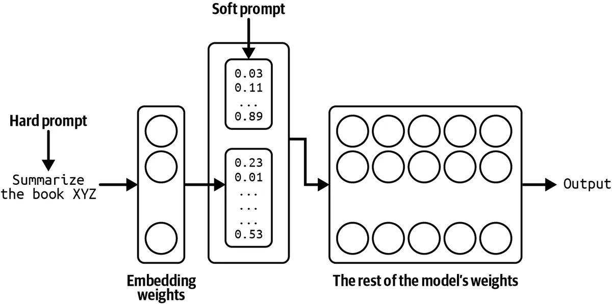Hard prompts are real tokens; soft prompts are learned vectors prepended to the embedded input while the rest of the model stays frozen

Prompt tuning (Lester et al., 2021) prepends k trainable vectors to the input embeddings only, at the first layer. It is the simplest variant and its headline result is scaling: with T5 models up to 11B parameters, prompt tuning closed the gap to full finetuning as model size grew. Prefix tuning (Li and Liang, 2021) prepends trainable key and value vectors at every layer's attention, giving the soft prompt more leverage at the cost of more parameters. P-tuning (Liu et al., 2021) inserts trainable vectors at arbitrary positions in the input and trains them through a small LSTM or MLP encoder to stabilize optimization, particularly for smaller models.

Soft prompts occupy a few positions of context on every request and have no inference overhead beyond that. They are attractive when you must serve many tasks from one frozen model and cannot change the weights at all. Their drawbacks are sensitivity to initialization and learning rate, weaker results on small models, and opacity: when a soft prompt misbehaves there is nothing to read. In practice, LoRA has displaced them for most application work.

Model merging and multi-task finetuning

Suppose you want one model that is good at two things. The direct route is multi-task finetuning: either train on both datasets simultaneously (mix them in one run) or sequentially (finetune on task A, then on task B). Simultaneous training needs both datasets at once and a balancing recipe; sequential training risks the second task overwriting the first. Model merging offers a third route that needs no training at all: take two models already finetuned for A and B and combine their weights.

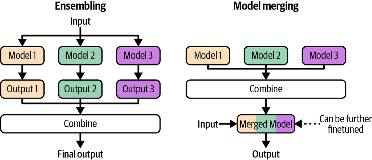Ensembling combines model outputs at inference time; model merging combines the models themselves into one that can be finetuned further

Merging differs from ensembling. An ensemble runs all constituent models and combines their outputs, paying full inference cost for each model. A merge produces a single model whose inference cost is that of one constituent, and the merged model can itself be finetuned further. Merging has become a staple of the open-weight community because it needs no GPUs, no gradients and no training data, only checkpoints that share a common ancestor; it is also useful for on-device deployment (one model instead of several) and for federated settings where models trained on separate data are combined without sharing the data.

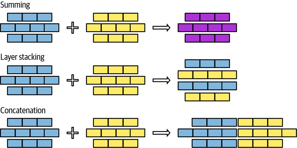Three ways to merge models: summing weights, stacking layers, and concatenating

The book organizes merging into three mechanical operations: summing corresponding weights, stacking layers, and concatenating.

Summing

Linear combination and task vectors. The simplest merge averages corresponding weights, optionally with per-model coefficients. Ilharco et al. (2022) reframed this in terms of task vectors: for a finetuned model M_A derived from base B, the task vector is τ_A = W_A − W_B, the direction in weight space that encodes task A. Task vectors support arithmetic. Adding τ_A + τ_B to the base gives a model with both skills; subtracting a task vector removes a behaviour (for example, un-learning toxic generation); scaling one adjusts its strength. Because all models share the base, weight-space directions remain roughly compatible, which is why naïve averaging works at all.

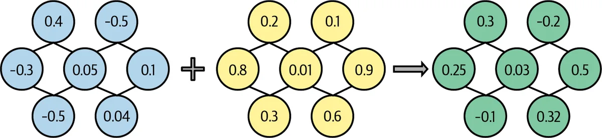Linearly combining two layers: each pair of corresponding weights is averaged

Spherical interpolation (SLERP) treats the two weight vectors as points on a sphere and interpolates along the arc rather than the chord, preserving their norm; linear interpolation between two directions shortens the result. SLERP merges two models at a time, so several models are merged pairwise.

Pruning redundant parameters: TIES and DARE. Summing task vectors naïvely creates interference: most entries of a task vector are small noise, and where two vectors disagree in sign they cancel. TIES-Merging (Yadav et al., 2023) works in three steps: trim each task vector to its top-k% largest-magnitude entries (the paper found keeping around 20% best), elect a sign per parameter by majority of the surviving magnitudes, and merge by averaging only the entries that agree with the elected sign. DARE (Yu et al., 2023) takes a randomized approach: drop a large random fraction p of each task vector's entries (often 90% or more) and rescale the survivors by 1 / (1 − p) so the expected update is unchanged; the sparsified vectors interfere far less and merging them is nearly free of quality loss.

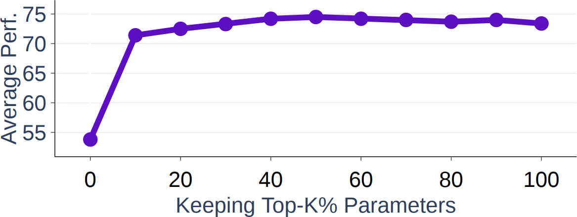Pruning task vectors: keeping only the top 20% of parameters by magnitude gives the best merged performance

Layer stacking

Stacking methods build a new architecture out of existing layers instead of averaging within a layer. The resulting model is usually larger than its parents and typically needs some further training to settle.

Franken-merging (passthrough). Take layers from different models and concatenate them depth-wise: say, layers 1 to 24 of model A followed by layers 17 to 40 of model B. Goliath-120B was made from two Llama 2 70B finetunes this way. Surprisingly, these stitched models often work without retraining, because adjacent transformer layers in the same family operate on roughly compatible residual streams.

Depth upscaling. SOLAR 10.7B (Kim et al., 2023) duplicated a 32-layer 7B model, removed the last 8 layers of the first copy and the first 8 of the second, stacked the remaining 24 + 24 into a 48-layer model, and continued pretraining. The result outperformed both its 7B parent and larger mixture-of-experts models of the time at a fraction of the training cost of a new 10B model.

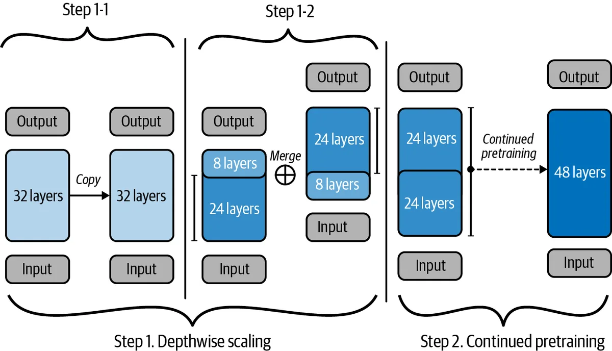Depthwise scaling: copy a 32-layer model, merge the copies into 48 layers, then continue pretraining

Mixture-of-experts upcycling. Sparse upcycling (Komatsuzaki et al., 2022) converts a dense model into an MoE: the attention weights are copied once, the feed-forward block is duplicated into N experts, a router is added and trained from scratch, and the whole thing is trained further. Because each expert starts from the same trained MLP, the model begins at the dense model's quality instead of from zero, and the experts specialize during continued training. Community merges that bolt several finetuned 7B models together as "experts" behind a fresh router are a cheaper, cruder version of the same idea.

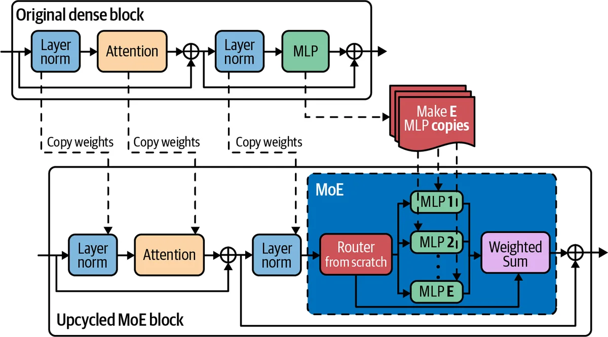Upcycling a dense block into a mixture-of-experts block: the attention weights are copied and the MLP is duplicated into experts behind a router trained from scratch

Concatenation

Concatenation joins parameters along a dimension rather than adding them. The concrete case is LoRA adapters: concatenating an adapter of rank r₁ with one of rank r₂ produces a single adapter of rank r₁ + r₂ whose update is the sum of the two, which is mathematically equivalent to applying both adapters. It is a tidy way to package two adapters as one, but it saves no parameters relative to keeping them separate, so it is less used than summing or stacking.

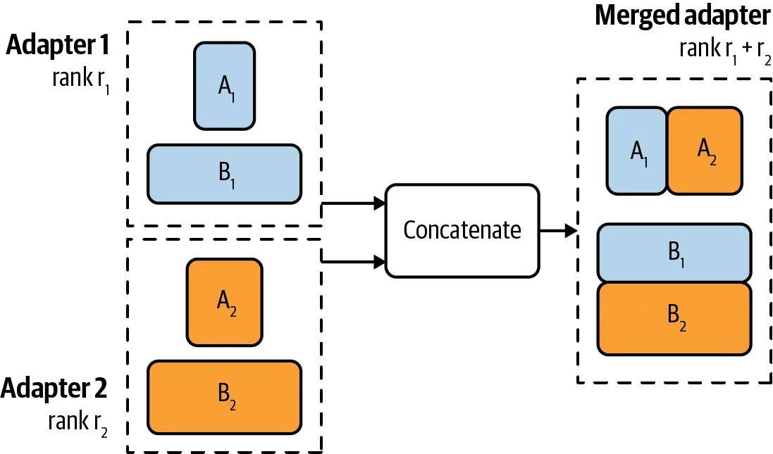Concatenating two LoRA adapters of rank r1 and r2 gives an adapter of rank r1 + r2

Merging in practice

Method	Needs training?	Output size	Works best when	Watch out for
Linear / task arithmetic	No	Same as parents	Few models, same base, related tasks	Interference, quality dilution with many models
SLERP	No	Same as parents	Exactly two models	Pairwise only
TIES / DARE	No	Same as parents	Many task vectors from one base	Trim and drop rates need tuning
Franken-merge	Usually a little	Larger	Parents from the same family	Unpredictable; must evaluate
Depth upscaling	Yes (continued pretraining)	Larger	Cheap route to a mid-size model	Still needs real training compute
MoE upcycling	Yes	Much larger (sparse)	Scaling capacity without pretraining from zero	Router needs training; serving complexity
LoRA concatenation	No	Sum of adapter ranks	Packaging adapters	No parameter savings

Tooling such as mergekit implements all of these behind a configuration file, which is why merging has been so popular on open-model leaderboards. The caveat is evaluation: a merge can look good on a benchmark and behave erratically on real traffic, so treat merged checkpoints like any other candidate model and run your own evaluation suite.

Finetuning tactics

Choosing a base model and a development path

The base model decision is usually the biggest single determinant of how a finetuning project turns out, and it depends on which of two paths you are on.

Progression path. Start by testing the task with the cheapest models to establish feasibility, move to the strongest model you can afford to find the ceiling, then finetune the smallest model that can plausibly reach your target. Each step informs the next: if even the strongest model cannot do the task with a good prompt, more data will not fix a 7B model. Finetuning mid-size models (7B to 13B class) is the common sweet spot because they are cheap to train, fit on one or two GPUs for LoRA, and retain enough capacity to learn non-trivial behaviours.

Distillation path. Use a large model to generate (or label) training data, then finetune a small model on it. This is faster to start when you lack labelled data and gives you a small, fast deployable from day one; its risk is that the student inherits the teacher's mistakes and style quirks (more on this in the data chapter). Check the teacher's license: several providers forbid using their outputs to train competing models.

Beyond size, evaluate candidate bases on in-domain capability (a code-specialized base for a code task), tokenizer fit for your language or data, context length, license terms for commercial use and redistribution, and the ecosystem of adapters and quantized builds you can reuse. The better the base fits, the less data and the lower the rank you need.

Choosing a method

Situation	Reasonable default
First finetuning project, data in hand, API provider fine	Managed finetuning API (OpenAI, Google, Mistral, Together and others): no infra, limited control, usually LoRA-style under the hood
Open-weight model, one or two GPUs	LoRA on all linear layers, r = 16, BF16 base, activation recomputation
Open-weight model, consumer GPU or 70B class on one node	QLoRA with NF4 base
Hard domain shift, large data, GPUs to spare, target-task quality is everything	Full finetuning, then compare against LoRA on your held-out capabilities
Many tasks or tenants, one deployment	LoRA per task, multi-LoRA serving
Several finetuned checkpoints already exist	Merge (TIES or DARE) and evaluate before training anything new

Frameworks such as Hugging Face PEFT and TRL, Axolotl, LLaMA-Factory, Unsloth and LitGPT bundle sensible defaults for all of these; start from a framework's recipe for your base model rather than from scratch.

Hyperparameters

Finetuning needs far less hyperparameter search than pretraining because the model starts from a good solution. Four knobs account for most of the outcomes.

Learning rate. The most important one. Full finetuning uses small rates, typically 1 × 10⁻⁵ to 5 × 10⁻⁵, because large steps destroy pretrained representations. LoRA tolerates and usually needs higher rates, around 1 × 10⁻⁴ to 3 × 10⁻⁴, because the adapters start at zero and the base is protected. A cosine or linear decay with a short warmup (a few percent of steps) is standard. Read the loss curve: a rate too high shows as a loss that spikes or plateaus early; too low shows as a loss that is still falling smoothly when training ends.

Batch size. Larger batches give smoother gradient estimates and better hardware utilization but cost memory; small batches are noisy. When the batch you want does not fit, gradient accumulation sums gradients over several micro-batches before each optimizer step, so a micro-batch of 4 with 8 accumulation steps behaves like a batch of 32 for optimization purposes while using the memory of 4. Effective batch sizes of 16 to 64 sequences are typical for instruction finetuning.

Number of epochs. How many passes over the data. Small datasets (a few thousand examples) often benefit from several epochs, four to ten being common; large datasets (hundreds of thousands or more) usually need only one or two. The signal to watch is divergence between training and validation loss: when training loss keeps dropping while validation loss rises, the model is memorizing. Stop there or regularize.

Prompt loss weight. An instruction example is a prompt followed by a response. The training loss can be computed over all tokens or only over the response tokens. Weighting the prompt tokens at zero teaches the model to generate responses, not to reproduce prompts, and is the usual choice; a small positive weight (OpenAI's legacy API defaulted to 0.1) can help when prompts are long and informative and the response is short. If your framework calls this "train on inputs" or "completion-only loss", it is the same knob.

Hyperparameter	Full finetuning	LoRA / QLoRA	How to tell it is wrong
Learning rate	1e-5 to 5e-5	1e-4 to 3e-4	Spikes or early plateau (too high); slow steady descent at the end (too low)
Effective batch size	16 to 64	16 to 64	Very noisy loss (too small); poor generalization with tiny data (too large)
Epochs	1 to 3 for large data; more for small	Same	Validation loss rising while training loss falls
Prompt loss weight	0 to 0.1	Same	Model parrots instructions or fails on long-prompt tasks
LoRA rank r	–	8 to 64	Underfits on hard shift (too low); no gain for the memory (too high)
LoRA alpha	–	r or 2r	Usually leave fixed; tune learning rate instead
Weight decay	0 to 0.1	0 to 0.1	Rarely decisive for short runs
Warmup	3 to 10% of steps	Same	Instability in the first few hundred steps

A reasonable starting recipe for LoRA on an instruction dataset is r = 16, α = 32, learning rate 2 × 10⁻⁴, effective batch 32, 3 epochs, cosine schedule with 3% warmup, loss on completion tokens only. Spend the experimentation budget on data inspection and on the evaluation set rather than on sweeping these.

Design trade-offs

Choosing between prompting, RAG, finetuning and distillation

Dimension	Prompt engineering	RAG	Finetuning	Distillation to a small model
Changes	Input	Input (adds retrieved context)	Weights	Weights of a different, smaller model
Fixes	Unclear instructions, simple format	Missing or changing knowledge, citations	Behaviour, format, style, consistency	Cost and latency at a quality target
Upfront cost	Minutes to days	Days to weeks (index, retriever, eval)	Weeks (data, training, eval)	Weeks (teacher generation plus finetuning)
Per-request cost	Highest tokens per call	Retrieval plus longer prompts	Shorter prompts, same model	Lowest
Knowledge freshness	None	Immediate	Frozen at training time	Frozen
Upgrade path when base improves	Free	Free	Retrain	Regenerate data and retrain
Failure mode	Model ignores instructions	Bad retrieval, context mis-use	Forgetting, over-fitting, stale behaviour	Imitates teacher style without its competence

Choosing a finetuning method

Dimension	Full finetuning	LoRA	QLoRA	Soft prompts	Merging
Trainable parameters	100%	~0.1 to 1%	~0.1 to 1%	< 0.01%	0
Training memory for a 7B model	> 100 GB (multi-GPU)	~16 to 24 GB	~6 to 10 GB	~16 GB	None (CPU)
Quality ceiling	Highest	Close on most tasks; behind on hard shifts	Slightly below LoRA	Lower on small models	Unpredictable; evaluate
Forgetting	Most	Less	Less	Least	Varies
Inference overhead	None	None merged; small unmerged	Base stays 4-bit or is dequantized	A few tokens of context	None
Multi-task serving	One copy per task	Shared base, swap adapters	Same	Shared base, swap prompts	One merged model

Interview angle

• When would you finetune instead of using RAG, and vice versa? Diagnose the failure. If the model lacks or mis-states facts, especially facts that change or must be cited, use RAG; finetuning is poor at injecting knowledge and can increase hallucination. If the model has the information but behaves badly (wrong format, inconsistent tone, ignores schema), finetune. Many production systems do both, finetuning on examples whose inputs already contain retrieved context.

• Estimate the GPU memory to fully finetune a 7B model with Adam. Weights 14 GB in BF16, gradients 14 GB, two Adam states 28 GB in BF16, for 56 GB before activations; with FP32 master weights and FP32 optimizer states (the standard mixed-precision recipe) it is about 112 GB. Add activations, which depend on batch and sequence length and can exceed the weights for long sequences. So full finetuning of 7B needs multiple 80 GB GPUs or heavy sharding, while LoRA fits on one.

• Why does LoRA save memory, and why does it add no inference latency? Only the low-rank matrices A and B are trainable, so gradients and optimizer states exist only for them; the frozen base needs none, cutting optimizer memory by orders of magnitude. After training, BA is added into W to give one dense matrix, so inference runs the same kernels as the base model. Kept unmerged, the small extra matmul lets many adapters share a base.

• Explain QLoRA and what it does not do. The frozen base is stored in 4-bit NF4 (quantile-spaced levels that fit normally distributed weights), dequantized to BF16 per matmul; LoRA adapters in BF16 are the only trainable parameters; double quantization shrinks the scale factors; paged optimizers absorb memory spikes. It makes a 65B finetune fit on a 48 GB GPU. It does not speed up training (dequantization adds work) and it does not by itself quantize the final model for serving.

• Compare FP16 and BF16. Why did BF16 win for LLMs? Both are 16 bits. FP16 has 5 exponent bits and 10 mantissa bits: more precision, but a maximum around 65,504, so gradients overflow and small values underflow unless you use loss scaling. BF16 has 8 exponent bits (FP32's range) and 7 mantissa bits. Training is far more sensitive to range than to precision, so BF16 removes the overflow failure mode at a precision cost the network tolerates.

• A finetuned model nails the target task but got worse at general instruction following. What happened and what would you do? Catastrophic forgetting: the updates overwrote representations other behaviours used. Mitigations: lower learning rate or fewer epochs, LoRA instead of full finetuning (it forgets less), mix a small fraction of general instruction data into the training set (replay), and extend the evaluation suite so the regression is caught before shipping.

• How would you serve fifty customer-specific variants of one model cheaply? Train a LoRA adapter per customer, keep the base model loaded once, and use a multi-LoRA serving engine (vLLM, TGI, LoRAX) that batches requests across adapters and pages adapters in and out. Each adapter is tens of megabytes versus tens of gigabytes for a full copy, and per-token overhead is a small extra low-rank matmul.

• What is a task vector and how do TIES and DARE improve on averaging them? A task vector is finetuned weights minus base weights: the direction encoding a task. Adding several to the base merges tasks without training, but noise entries and sign conflicts interfere. TIES trims each vector to its largest entries, elects a sign per parameter by majority, and averages only agreeing entries. DARE randomly drops most entries and rescales the rest so the expected update is preserved; sparse vectors overlap less and merge cleanly.

• Which hyperparameters matter most in finetuning and how do you set them? Learning rate first (1e-5 to 5e-5 for full finetuning, around 1e-4 to 3e-4 for LoRA), read from the loss curve. Then epochs, watched through train-versus-validation divergence; effective batch size, reached with gradient accumulation if memory is short; and prompt loss weight, usually zero so the loss covers only response tokens. LoRA rank and alpha come after; data quality beats all of them.

Pitfalls and misconceptions

• "Finetune to teach the model our documentation." Finetuning is a weak and risky way to add facts; it tends to teach confidence before content. Use retrieval for knowledge and finetune, if at all, to teach the model how to use retrieved context.
• Treating the training run as the project. The run is hours; the data collection, cleaning, formatting and evaluation around it are weeks. Teams that skimp on the evaluation set cannot tell whether finetuning helped.
• Finetuning before a serious prompting baseline. If a strong prompt with a few examples gets 90% of the way, a finetune may buy little and costs a maintenance stream. Measure the gap first.
• Assuming PEFT equals full finetuning quality everywhere. LoRA matches full finetuning on most adaptation tasks but trails it on hard domain shifts with lots of data; it compensates by forgetting less. Pick by measuring both on target and held-out capabilities.
• Confusing LoRA alpha with the learning rate. Alpha scales the update by α / r; doubling r at fixed α halves each component's effect. Fix α to r or 2r and tune the learning rate rather than fighting both.
• Evaluating only the target task. Regression on general capabilities, safety behaviour and format adherence is the common failure. Keep a held-out suite that reflects everything you still need.
• Using the wrong chat template or training on prompt tokens by accident. Both silently produce a model that looks trained but misbehaves at inference. Decode a few formatted examples and confirm the loss mask before every run.
• Expecting quantization to be free. INT8 weight-only is close to free; INT4 costs measurable quality on small models; activation quantization must deal with outlier channels. Benchmark the quantized artefact, not the BF16 one you trained.

Key terms

Term	Meaning
Transfer learning	Reusing knowledge learned on one task to learn another from less data; finetuning is its weight-updating form
Feature-based transfer	Freezing the pretrained model and training a separate model on its outputs
Catastrophic forgetting	Loss of previously learned capabilities when a network is trained on new data
Supervised finetuning (SFT)	Training on (prompt, response) pairs to imitate the responses
Activation	An intermediate output of a layer, stored during the forward pass for use in the backward pass
Optimizer state	Per-parameter statistics an optimizer keeps between steps; Adam keeps two (first and second moment)
Activation recomputation (gradient checkpointing)	Storing a subset of activations and recomputing the rest in the backward pass to save memory
Mixed precision training	Computing in FP16 or BF16 while keeping FP32 master weights and optimizer states
BF16	16-bit float with 8 exponent and 7 mantissa bits; FP32's range at half the size
Quantization	Mapping values to a lower-precision format using a scale and rounding; PTQ is applied after training, QAT during
Outlier features	A few activation channels with very large magnitudes that break naïve per-tensor quantization
NF4	4-bit NormalFloat, with levels at the quantiles of a normal distribution; QLoRA's base-weight format
PEFT	Parameter-efficient finetuning: adapting a model by training a small number of (usually new) parameters
Adapter	A small trainable module inserted into a frozen network; Houlsby adapters are bottleneck MLPs with a skip connection
LoRA	Low-Rank Adaptation: learning ΔW = BA with small rank r in parallel to a frozen W, mergeable after training
Rank (r) and alpha (α)	LoRA's capacity and scaling hyperparameters; the update is scaled by α / r
Intrinsic dimension	The dimensionality of the subspace in which a task's finetuning solution lies; low for pretrained LLMs
Soft prompt	Trainable continuous vectors prepended to the input (prompt tuning) or to each layer (prefix tuning)
Task vector	Finetuned weights minus base weights; the weight-space direction encoding a task
TIES / DARE	Merging methods that reduce interference by trimming and sign-electing (TIES) or randomly dropping and rescaling (DARE) task-vector entries
Franken-merge / depth upscaling	Building a deeper model by stacking layers from existing models, with or without continued training
Sparse upcycling	Converting a dense model into a mixture of experts by duplicating the MLP into experts behind a new router
Gradient accumulation	Summing gradients over several micro-batches before an optimizer step to emulate a larger batch
Prompt loss weight	The weight given to prompt tokens in the training loss; zero means loss only on response tokens

Further reading

• AI Engineering, Chapter 7 (Finetuning); companion material at https://github.com/chiphuyen/aie-book
• Hu et al., "LoRA: Low-Rank Adaptation of Large Language Models" (2021): https://arxiv.org/abs/2106.09685
• Dettmers et al., "QLoRA: Efficient Finetuning of Quantized LLMs" (2023): https://arxiv.org/abs/2305.14314
• Houlsby et al., "Parameter-Efficient Transfer Learning for NLP" (2019): https://arxiv.org/abs/1902.00751
• Lester, Al-Rfou and Constant, "The Power of Scale for Parameter-Efficient Prompt Tuning" (2021): https://arxiv.org/abs/2104.08691
• Li and Liang, "Prefix-Tuning: Optimizing Continuous Prompts for Generation" (2021): https://arxiv.org/abs/2101.00190
• Aghajanyan, Zettlemoyer and Gupta, "Intrinsic Dimensionality Explains the Effectiveness of Language Model Fine-Tuning" (2020): https://arxiv.org/abs/2012.13255
• Biderman et al., "LoRA Learns Less and Forgets Less" (2024): https://arxiv.org/abs/2405.09673
• Gekhman et al., "Does Fine-Tuning LLMs on New Knowledge Encourage Hallucinations?" (2024): https://arxiv.org/abs/2405.05904
• Ilharco et al., "Editing Models with Task Arithmetic" (2022): https://arxiv.org/abs/2212.04089
• Yadav et al., "TIES-Merging: Resolving Interference When Merging Models" (2023): https://arxiv.org/abs/2306.01708
• Yu et al., "Language Models are Super Mario: Absorbing Abilities from Homologous Models as a Free Lunch" (DARE, 2023): https://arxiv.org/abs/2311.03099
• Kim et al., "SOLAR 10.7B: Scaling Large Language Models with Simple yet Effective Depth Up-Scaling" (2023): https://arxiv.org/abs/2312.15166
• Komatsuzaki et al., "Sparse Upcycling: Training Mixture-of-Experts from Dense Checkpoints" (2022): https://arxiv.org/abs/2212.05055
• Dettmers et al., "LLM.int8(): 8-bit Matrix Multiplication for Transformers at Scale" (2022): https://arxiv.org/abs/2208.07339
• Micikevicius et al., "Mixed Precision Training" (2017): https://arxiv.org/abs/1710.03740
• Rajbhandari et al., "ZeRO: Memory Optimizations Toward Training Trillion Parameter Models" (2019): https://arxiv.org/abs/1910.02054
• Hugging Face PEFT documentation: https://huggingface.co/docs/peft