Training a model happens a few times; inference happens on every request for the life of the product. For most deployed AI systems the inference bill dwarfs the training bill, and the latency a user feels is almost entirely inference latency. Inference optimization is the discipline of making a given model answer faster, serve more users per accelerator and cost less per token, ideally without changing what it outputs.

This chapter builds the mental model first: why autoregressive generation is bottlenecked on memory bandwidth rather than arithmetic, how to measure latency and throughput honestly, and what accelerators actually provide. It then walks the two layers at which you can intervene. Model-level optimizations change the model or how its computation is scheduled (quantization, pruning, distillation, attention redesign, KV cache management, speculative decoding, compiled kernels). Service-level optimizations change how requests are scheduled onto hardware (batching, prefill/decode disaggregation, prompt caching, parallelism). Even if you only call a hosted API, this chapter explains your bill, your latency percentiles and why prompt caching discounts exist.

In one minute

• Generation has two phases. Prefill processes the whole prompt in parallel and is compute-bound; it sets time to first token. Decode emits one token per forward pass and is memory-bandwidth-bound at small batch sizes; it sets time per output token.
• Whether a workload is compute- or bandwidth-bound is decided by arithmetic intensity (FLOPs per byte moved) against the hardware's ops:byte ratio. The roofline model draws this as a chart; decode lives under the sloped part of the roof.
• Measure latency as TTFT, TPOT and total latency, in percentiles (p50, p90, p99), on realistic prompts. Measure throughput as tokens per second and requests per second, and prefer goodput: requests per second that meet the latency SLO.
• MFU and MBU tell you how much of the chip's compute or bandwidth you are using; low MFU in decode is expected, low MBU is a real inefficiency.
• Accelerators are bought for memory bandwidth and capacity as much as FLOP/s; the memory hierarchy (SRAM, HBM, host DRAM) is what FlashAttention, tiling and operator fusion exploit.
• Model-level wins: weight-only quantization to INT8 or INT4 cuts bytes per token; MQA/GQA and PagedAttention shrink and pack the KV cache; FlashAttention makes exact attention IO-efficient; speculative decoding produces several tokens per target-model pass with unchanged output distribution.
• Service-level wins: continuous batching keeps the GPU full while requests of different lengths come and go; prompt caching reuses the KV cache of shared prefixes; prefill/decode disaggregation and tensor, pipeline, replica and context parallelism match phases and model sizes to hardware.
• Optimizations compound. A reference PyTorch pipeline took Llama 7B from about 25 to about 245 tokens per second by stacking compilation, INT8, INT4 and speculative decoding. Start with a serving engine that has these built in (vLLM, TensorRT-LLM, TGI, SGLang) before writing kernels.

Understanding inference optimization

Inference servers and services

An inference server loads a model onto hardware and executes forward passes; it worries about kernels, batching and memory. An inference service wraps one or more servers with an API, routing, autoscaling, authentication and billing. Hosted model APIs are inference services operated by the model provider; self-hosting means running both yourself with an engine such as vLLM, TensorRT-LLM, Hugging Face TGI or SGLang. The split matters for this chapter because most techniques below live in the server, but the metrics that matter are observed at the service boundary.

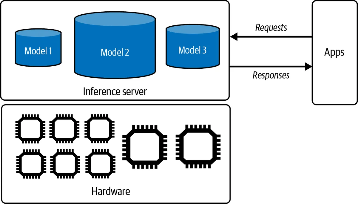An inference server hosts models on hardware and serves requests from applications

Who optimizes depends on where you sit. Model providers and self-hosters control everything from kernels to schedulers. API users control prompt length, output length, streaming, batching their own requests, model choice and whether they exploit prompt caching; the rest is the provider's job. Both need the same vocabulary.

Computational bottlenecks

Every operation in a forward pass needs some number of floating-point operations and some number of bytes moved between memory and the compute units. Its arithmetic intensity is the ratio: FLOPs per byte. A chip has a peak FLOP/s and a peak memory bandwidth (bytes per second); their ratio is the chip's ops:byte ratio, the intensity at which compute and memory take equal time. An operation with intensity above that ratio is compute-bound: the arithmetic units are the bottleneck and faster memory would not help. One below it is memory-bandwidth-bound: the units sit idle waiting for data, and more FLOP/s would not help.

An NVIDIA H100 SXM delivers roughly 990 dense TFLOP/s in BF16 against about 3.35 TB/s of HBM bandwidth, an ops:byte ratio near 300. An A100 is about 312 TFLOP/s against 2 TB/s, a ratio near 150. These are large numbers: an operation has to do hundreds of FLOPs for every byte it touches to keep the chip busy.

Now look at what a transformer does during generation.

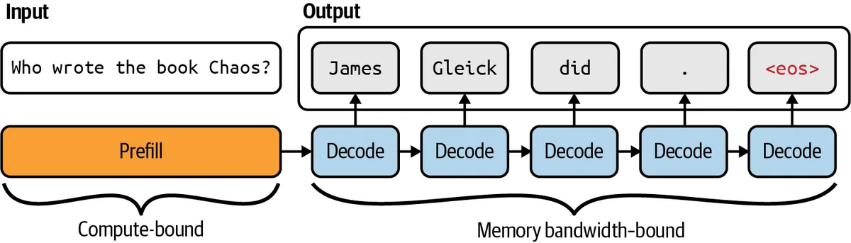Prefill processes the whole prompt in parallel and is compute-bound; decode generates one token at a time and is memory-bandwidth-bound

Prefill. All prompt tokens go through the model at once. Each weight matrix is read from memory once and multiplied against a matrix with as many rows as there are tokens, so the FLOPs per byte of weights scale with prompt length. For prompts of hundreds or thousands of tokens, prefill is compute-bound. It also produces the KV cache (the key and value vectors of every prompt token at every layer) and the first output token.

Decode. Each step feeds exactly one new token per sequence through the model. Every weight matrix must be read from HBM again, but it is multiplied against a single row. For a 70B model in BF16 that is 140 GB of weights read to produce one token per sequence, plus the whole KV cache. The arithmetic intensity is tiny, so decode at batch size one is almost perfectly memory-bandwidth-bound: tokens per second ≈ bandwidth ÷ bytes read per step. On an H100, 3.35 TB/s ÷ 140 GB gives an upper bound around 24 tokens per second for a single 70B BF16 sequence, regardless of how fast the tensor cores are.

Batching changes the picture. With B sequences decoding together, the weights are read once per step and applied to B rows, so intensity rises with B. Decode becomes compute-bound only at large batch sizes (hundreds of sequences for big models), and even then the KV cache reads, which are per-sequence and not shared, keep it bandwidth-heavy. This is why almost every serving trick is about one of three things: read fewer bytes per step (quantization, smaller KV cache), amortize the bytes over more useful work (batching, speculative decoding), or avoid redundant work entirely (KV cache, prompt caching).

Online, batch and streaming inference

Online inference serves requests as they arrive with a latency target; chat, copilots and interactive agents live here. Batch inference processes a large set of requests with no per-request latency requirement: nightly classification of yesterday's tickets, generating embeddings for a corpus, synthetic data generation, offline evaluation. Batch workloads can run at maximum batch size and utilization and tolerate queues, so they are far cheaper per token; providers reflect this with batch APIs that trade a turnaround window (often up to 24 hours) for a substantial discount (OpenAI's Batch API halves the price). If a workload can wait, let it.

Streaming returns tokens as they are generated instead of after the last one. It does not change total latency but transforms perceived latency: the user starts reading after TTFT instead of after TTFT plus the whole generation. Streaming also changes what you can do with output guardrails, since you cannot inspect a complete response before showing its beginning.

Inference APIs

Hosted APIs expose the same primitives with small differences that affect optimization. A completion or chat endpoint accepts a prompt or a message list and generation parameters (max tokens, temperature, stop sequences); streaming is a flag; structured output and tool-calling modes constrain decoding. Pricing is per input token and per output token, with output tokens several times more expensive because decode is the bandwidth-bound phase; prompt caching and batch modes are discounts for workloads the provider can serve more efficiently. Knowing which phase each parameter touches is the user-side version of inference optimization: a long system prompt costs prefill compute (and money) on every call unless cached; a large max-tokens budget that the model actually uses costs decode time on every call.

Inference performance metrics

Latency

Latency is what one user feels. For autoregressive generation it decomposes into pieces that have different causes and different fixes.

Metric	Definition	Governed by	Typical lever
TTFT (time to first token)	Request sent to first token received	Queueing plus prefill, so prompt length and compute	Shorter prompts, prompt caching, more compute, scheduling priority
TPOT (time per output token)	Average interval between subsequent tokens	Decode, so bytes per step and memory bandwidth	Quantization, smaller KV cache, speculative decoding, less batching
Total latency	TTFT + TPOT × number of output tokens	Both, plus output length	Cap or shorten outputs; everything above
Time to publish	When the user actually sees output, including any post-processing, guardrails or buffering	Pipeline design	Stream; move checks off the critical path

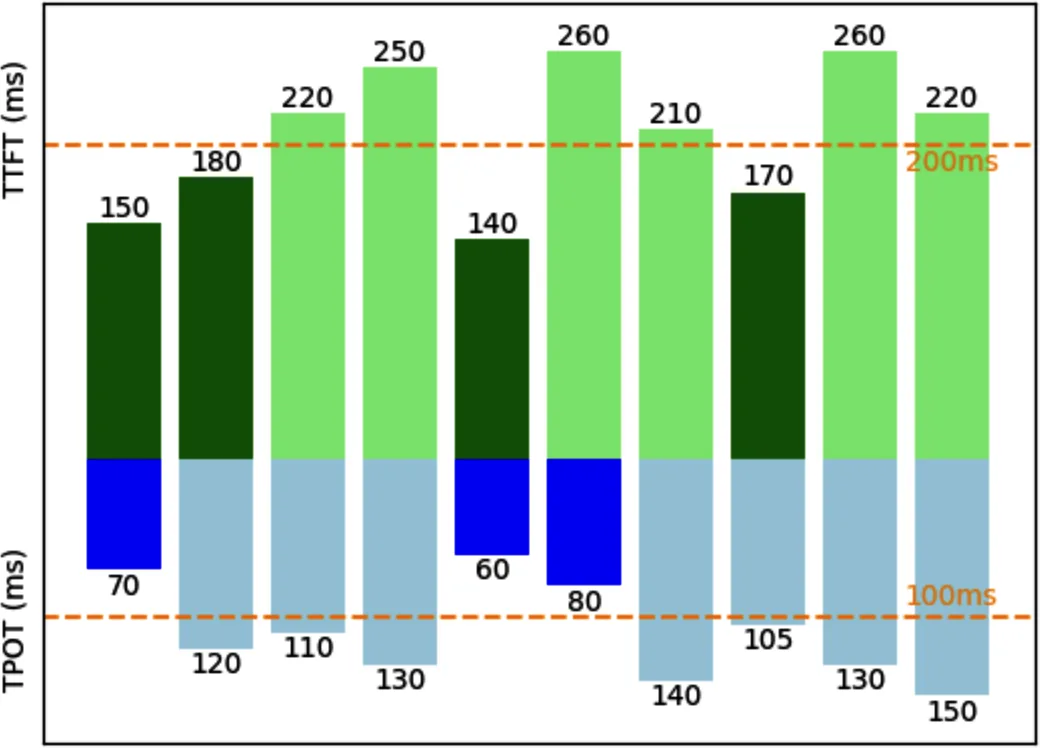Time to first token and time per output token: two systems can trade one against the other

TTFT and TPOT trade against each other in a loaded system. Scheduling a new request's prefill promptly improves its TTFT but stalls the decode steps of requests already in flight, raising their TPOT; batching more aggressively improves TPOT per dollar but queues new arrivals. A system tuned for chat might target TTFT under half a second and TPOT around 20 to 50 ms, which is faster than people read; a system generating long documents for later consumption can tolerate much worse TPOT if its throughput is high.

Two measurement habits matter. Report percentiles, not averages. Latency distributions have long tails (a few long prompts, a few slow batches, a queue spike), and the p99 is what your angriest users experience; an average hides a p99 ten times the median. Measure with realistic inputs. TTFT depends on prompt length and TPOT on batch load, so a benchmark with short prompts and no concurrency says nothing about production. Record input and output token counts alongside every latency sample so you can normalize.

Throughput and goodput

Throughput is what the operator pays for. Tokens per second can mean output tokens (what decode produces) or total tokens including prompt tokens (what the system processes); pick one and label it. Requests per second (or per minute) is the service-level view, and it depends heavily on request size: a system doing 1,000 tokens per second serves 100 ten-token requests or one 1,000-token request. Cost per token is throughput's inverse: fixed hardware cost per hour divided by tokens per hour.

Throughput and latency pull in opposite directions. Larger batches raise tokens per second by amortizing weight reads across more sequences but make each sequence's steps slower and queue new arrivals. The honest metric is therefore goodput: the number of requests per second (or tokens per second) that meet the latency SLO. A configuration that doubles raw throughput while pushing p90 TTFT past the SLO has lowered goodput. Capacity planning and autoscaling should be done on goodput, not on peak tokens per second.

Utilization: MFU and MBU

Model FLOP/s utilization (MFU) is the ratio of the FLOP/s the model actually achieves to the hardware's peak FLOP/s. Training runs reach 30 to 50% on well-tuned clusters. Inference MFU is often far lower, and during decode that is not an engineering failure: the workload is bandwidth-bound, so most FLOP capacity is structurally idle.

Model bandwidth utilization (MBU) is the matching metric for bandwidth: bytes actually moved per second (model weights plus KV cache per step, times steps per second) divided by peak memory bandwidth. In decode, MBU is the metric that tells you whether the serving stack is efficient; 70 to 80% is good, and the gap to 100% is kernel overhead, launch latency and synchronization. If MBU is high and the token rate is still too low, the only ways forward are fewer bytes per step (quantization, KV compression, smaller model) or hardware with more bandwidth.

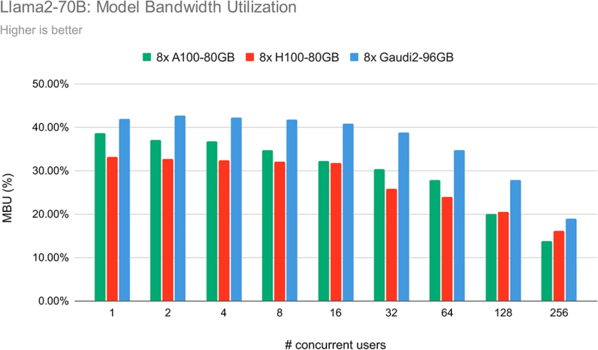Model bandwidth utilization for Llama 2 70B on different chips as concurrent users increase

MBU falls as concurrency rises: with more sequences per batch the same weight bytes serve more tokens, so the workload shifts toward compute and bandwidth utilization stops being the limiting factor. Plotting MBU against concurrent users shows where a given chip transitions from bandwidth-bound to compute-bound for a given model, which is exactly the batch size at which adding users stops being free.

The roofline model

The roofline chart plots attainable FLOP/s against arithmetic intensity on log-log axes. A sloped line from the origin has slope equal to memory bandwidth (attainable FLOP/s = bandwidth × intensity); a flat line at peak FLOP/s caps it. The two meet at the ops:byte ratio, the "knee". Any kernel sits at its intensity on the x-axis; its attainable performance is the roof above it.

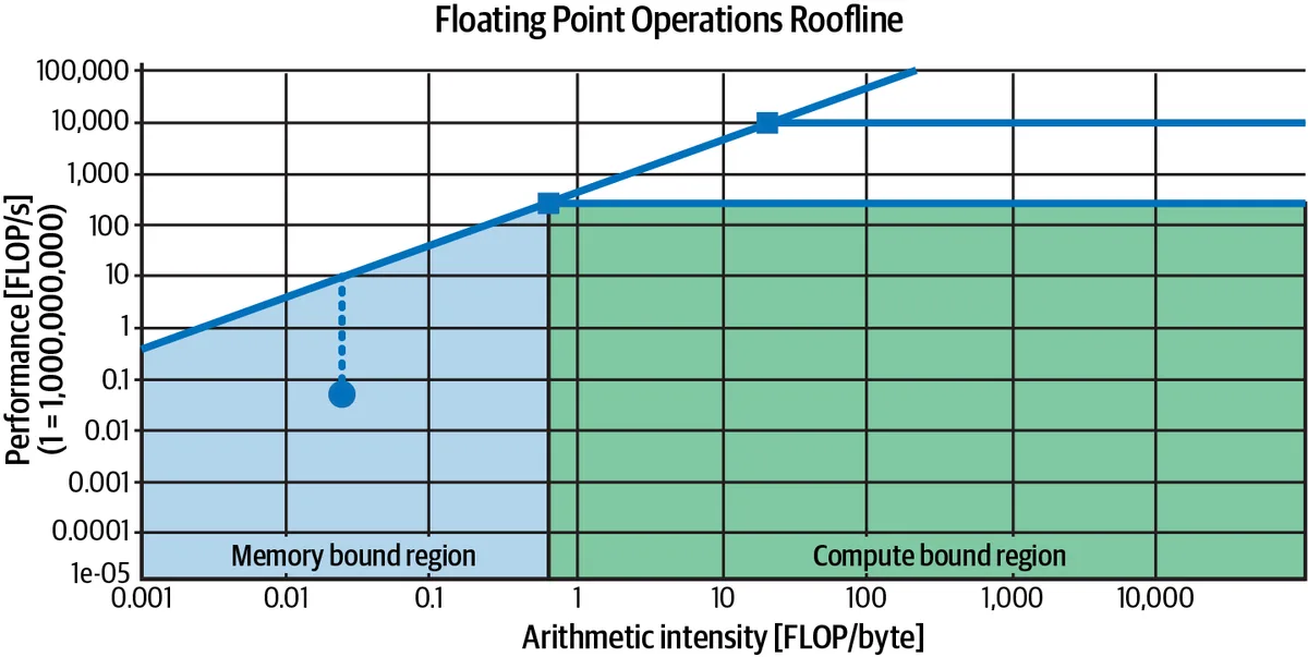A roofline chart: below the knee a workload is memory-bound, above it compute-bound

Decode at small batch sits far left of the knee under the sloped roof; nothing but more bandwidth or fewer bytes moves it up. Prefill and large-batch decode sit right of the knee under the flat roof, where better kernels and lower-precision tensor cores help. Every optimization in this chapter is a move on this chart: quantization shifts a kernel right (fewer bytes per FLOP); batching shifts decode right; FlashAttention lifts attention toward the roof by reducing wasted memory traffic; faster hardware raises one roof or the other.

AI accelerators

CPUs, GPUs and TPUs

A CPU spends its transistors on a few powerful cores with deep caches, branch prediction and out-of-order execution, which suits irregular control flow. A GPU spends them on thousands of simple arithmetic units organized into streaming multiprocessors, plus tensor cores that do small dense matrix multiplies in one instruction. Neural network inference is overwhelmingly dense matrix multiplication, which is why GPUs win by one to two orders of magnitude per dollar on this workload. Google's TPUs go further in the same direction: systolic arrays specialized for matrix multiplication, tightly coupled with XLA and the JAX/TensorFlow stack. Other accelerators (AWS Inferentia and Trainium, AMD Instinct MI300X, Intel Gaudi, Groq's LPU, Cerebras's wafer-scale engine) make different bets on memory type, interconnect and programmability, and all fight NVIDIA's CUDA ecosystem for software support.

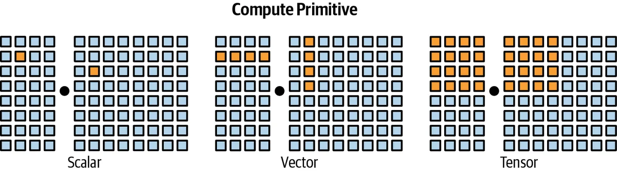Compute primitives: scalar, vector and tensor operations

Compute primitives explain the throughput ladder. Scalar units do one operation per instruction; vector (SIMD) units do the same operation across a short vector; tensor units do a small matrix multiply-accumulate per instruction. Tensor cores only help when the computation is shaped like dense matmul at the precision they support, which is a strong incentive to express everything as matmuls at 16 or 8 bits.

Memory hierarchy

The accelerator's memory system matters as much as its arithmetic.

Level	Typical capacity (H100 class)	Typical bandwidth	Notes
On-chip SRAM (registers, shared memory, L1/L2)	Tens of MB total	Tens of TB/s	Where tiles live during a kernel; far too small for weights
HBM (device memory)	80 GB (H100), 141 GB (H200), 192 GB (MI300X)	2 to 5 TB/s	Holds weights and KV cache; the bandwidth that bounds decode
Host DRAM	Hundreds of GB to TB	Tens to low hundreds of GB/s to the GPU over PCIe or NVLink-C2C	Offload target; far too slow for per-step weight reads
Other GPUs	n × 80 GB	NVLink ~900 GB/s per GPU; InfiniBand tens of GB/s across nodes	Enables tensor and pipeline parallelism

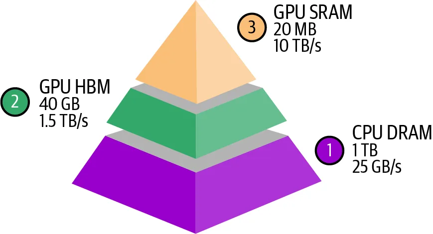The memory hierarchy: GPU SRAM is tiny but fast, HBM larger and slower, CPU DRAM larger and slower still

Two gaps drive design. The SRAM-to-HBM gap (roughly an order of magnitude in bandwidth, three orders in capacity) is why kernels tile computations to reuse data in SRAM and fuse operators so intermediate results never round-trip to HBM; FlashAttention is the famous case. The HBM-to-host gap is why models must fit in device memory, why KV cache capacity caps concurrency, and why offloading to CPU memory is a last resort that makes decode far slower.

FLOP/s, bandwidth, capacity and cost

When comparing accelerators for inference, four numbers matter and they are not interchangeable.

• Peak FLOP/s at the precision you will run. Tensor-core throughput roughly doubles with each halving of precision: on an H100 SXM, dense BF16 is about 990 TFLOP/s and FP8 about 1,980 TFLOP/s (NVIDIA's headline figures are double these because they assume 2:4 sparsity). This governs prefill and large-batch decode.
• Memory bandwidth. Governs decode at small and medium batch. The reason H200 and MI300X are attractive for LLM serving is bandwidth and capacity, not FLOP/s.
• Memory capacity. Decides whether the model fits on one device and how much KV cache (and therefore how many concurrent sequences) remains after the weights. A 70B model in BF16 needs 140 GB of weights alone, so it does not fit on one 80 GB GPU without quantization or tensor parallelism.
• Cost, including power. An H100 draws up to 700 W; a rack of them is a power and cooling problem before it is a capital one, and data centre power availability has become a real constraint on capacity. Compare chips on tokens per second per dollar for your workload shape, not on peak FLOP/s.

Chip	Memory	Bandwidth	Dense BF16	Notes
NVIDIA A100 80GB	80 GB HBM2e	~2.0 TB/s	~312 TFLOP/s	Workhorse of 2021 to 2023
NVIDIA H100 SXM	80 GB HBM3	~3.35 TB/s	~990 TFLOP/s	FP8 support; TMA and async copies used by FlashAttention-3
NVIDIA H200	141 GB HBM3e	~4.8 TB/s	~990 TFLOP/s	Same compute as H100; more memory for KV cache
AMD MI300X	192 GB HBM3	~5.3 TB/s	~1,300 TFLOP/s	Largest single-device memory of its generation

Figures are approximate vendor specifications; real throughput depends on the serving stack.

Selecting accelerators

Start from the workload, not the spec sheet. Long prompts and large offline batches are compute-heavy and reward FLOP/s. Interactive chat with short prompts and long outputs is decode-heavy and rewards bandwidth. Long contexts and high concurrency reward capacity because KV cache is what runs out first. Then check software: an engine that does not support a chip's quantized kernels or attention kernels forfeits most of its paper advantage. Finally weigh availability (lead times and cloud quotas have been binding constraints), interconnect (tensor parallelism needs NVLink-class bandwidth), and the precision roadmap (FP8 today, FP4 arriving).

The warning the book gives is worth repeating: do not buy on peak FLOP/s. For memory-bound decode, a chip with lower FLOP/s and higher bandwidth is faster, and for most chat workloads that is the regime you are in.

Model-level optimization: compression and attention

Model-level techniques change the model's weights, structure or kernels. They can be applied once and shipped with the model, and some of them (compression) can change outputs, so every one needs a quality evaluation on your task. This section covers the two biggest levers on bytes per step: shrinking the weights and shrinking the attention computation and its KV cache.

Quantization for inference

Quantization is covered in the finetuning chapter from the training side; here the question is what it buys at serving time. Weight-only quantization to INT8 halves the bytes read per decode step relative to BF16, and INT4 quarters them; because decode is bandwidth-bound, that translates almost directly into tokens per second at small batch, and it frees memory for more KV cache and therefore more concurrent sequences. Weight-and-activation quantization (W8A8, FP8) additionally lets the matmuls run on lower-precision tensor cores, which helps compute-bound prefill and large-batch decode. The KV cache can be quantized separately (INT8 or FP8 is common, INT4 with care), which attacks the other large per-step read.

Post-training methods differ in how they choose rounding. Round-to-nearest per channel works at INT8. At INT4, GPTQ uses second-order information on a calibration set to minimize layer output error; AWQ protects the small fraction of salient weights that activations amplify; SmoothQuant moves quantization difficulty from outlier-heavy activations into weights so both can be 8-bit. Formats such as GGUF (llama.cpp), GPTQ, AWQ and FP8 checkpoints are now standard artefacts, and serving engines ship kernels for each.

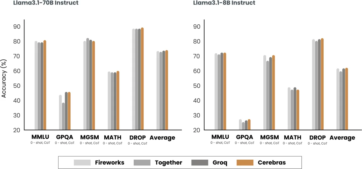The same open model served by different providers scores differently on benchmarks, because each provider quantizes and optimizes differently

The quality cost is real and uneven. INT8 weight-only is usually within noise; INT4 costs a measurable fraction of a point on benchmarks for large models and more for small ones, and it can hurt specific capabilities (long-context recall, maths) more than averages suggest. The same open model served by different providers scores differently on public benchmarks precisely because each provider picks its own quantization and kernels. Evaluate the quantized artefact you deploy, not the BF16 checkpoint you downloaded.

Pruning

Pruning removes parameters. Unstructured pruning zeroes individual weights by magnitude or by a sensitivity score; models tolerate high sparsity with modest quality loss, but dense hardware gains nothing from scattered zeros unless the sparsity pattern is one the hardware supports. NVIDIA's Ampere and later tensor cores support 2:4 structured sparsity (two of every four weights zero), which gives up to 2× matmul throughput and halves weight storage, and methods such as SparseGPT prune LLMs to this pattern in one shot. Structured pruning removes whole attention heads, neurons or layers, producing a genuinely smaller dense model that runs faster everywhere but typically needs finetuning to recover quality (Sheared-LLaMA and Minitron are examples of prune-then-retrain pipelines).

Pruning is less used for LLM serving than quantization because quantization is simpler, better supported and gives larger bandwidth savings per unit of quality lost. It becomes attractive when combined with retraining as a cheaper route to a small model than training one from scratch.

Distillation

Distillation (see the dataset chapter) trains a smaller student on a larger teacher's outputs or output distributions. For serving it is the most aggressive compression: a 7B student is not a cheaper 70B, it is a different model with its own cost profile, several times fewer bytes per step and fewer layers to traverse. The trade is a quality ceiling set by the student's capacity and the risk of imitating style over substance. Compression techniques stack: a common production recipe is distil into a smaller model, prune or shear it, then quantize the result to INT4 or FP8 for serving.

The KV cache

In decode, each new token must attend to every earlier token's keys and values at every layer. Recomputing them each step would make generation quadratic in sequence length; instead the KV cache stores them once (prefill writes the prompt's, each decode step appends one token's). The cache is the price of linear-time decode, and it is paid in memory.

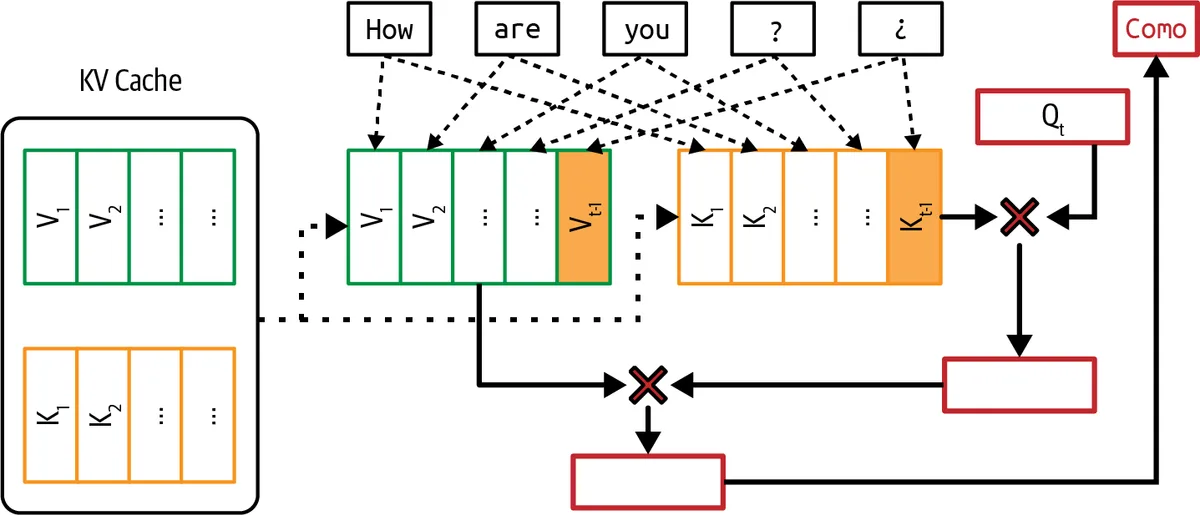The KV cache stores the key and value vectors of earlier tokens so each new token only computes its own

Its size per token is 2 (keys and values) × layers × KV heads × head dimension × bytes per value. For Llama 2 70B in BF16: 2 × 80 layers × 8 KV heads × 128 dims × 2 bytes = 327,680 bytes, about 320 KB per token. A 4,096-token sequence therefore holds about 1.34 GB of cache; a hundred concurrent sequences of that length need 134 GB, more than the 140 GB of weights leave on two 80 GB GPUs. Without GQA (Llama 2 7B has 32 KV heads but only 32 layers and a 4,096 hidden size) the figure is 512 KB per token, 2 GB per 4k sequence. The cache grows linearly with context length and with concurrency, and for long-context serving it, not the weights, is the binding memory constraint.

Lever	What it does to the KV cache	Where it acts
MQA / GQA	Fewer KV heads: 8× to 32× smaller cache	Model architecture (training time)
Sliding-window / local attention	Cache bounded by window size on those layers	Model architecture
Cross-layer attention	Adjacent layers share one cache	Model architecture
KV cache quantization	2× to 4× smaller per token	Serving engine
PagedAttention	Eliminates fragmentation and over-allocation	Serving engine
Eviction and compression	Drops or merges low-importance tokens	Serving engine, approximate
Prefix (prompt) caching	Shares cache across requests with a common prefix	Serving engine

Redesigning attention

Standard multi-head attention (MHA) gives every query head its own key and value heads, so the cache has one K and one V per head per layer. Multi-query attention (MQA) (Shazeer, 2019) shares a single K and V head across all query heads, shrinking the cache by the number of heads (32× for a 32-head model) at some quality cost. Grouped-query attention (GQA) (Ainslie et al., 2023) is the compromise: query heads are divided into groups that each share one KV head. Llama 2 70B uses 64 query heads and 8 KV heads, an 8× cache reduction with quality close to MHA, and most models since have adopted GQA. Because the KV cache is read on every decode step, these reductions improve TPOT and concurrency directly.

Local or sliding-window attention limits each token to attending over the previous w tokens, bounding both compute and cache for those layers at O(n·w) instead of O(n²); Mistral 7B used a 4,096-token window. Interleaving windowed layers with a few full-attention layers (as several 2024 models do) keeps long-range access while slashing cache. Cross-layer attention (Brandon et al., 2024) shares KV caches between adjacent layers, cutting cache size by the sharing factor with small quality loss. Character.AI reported combining MQA, cross-layer KV sharing and sliding windows on most layers to shrink their KV cache more than 20×, which is what let them serve very long chat histories cheaply.

Managing the KV cache in the serving engine

PagedAttention (Kwon et al., 2023, the core of vLLM) applies virtual-memory ideas to the cache. Earlier engines allocated one contiguous region per request sized for the maximum possible length, wasting memory to internal fragmentation (space reserved but never used) and external fragmentation (gaps between regions). PagedAttention splits each sequence's cache into fixed-size blocks mapped through a per-sequence block table, allocates blocks on demand, and lets sequences share blocks (for shared prefixes or for parallel samples from one prompt) with copy-on-write. Memory waste drops to a few percent and the engine can pack several times more sequences into the same HBM, which raises batch size and therefore throughput. Essentially every modern engine now uses a paged cache.

KV cache quantization stores K and V in INT8 or FP8 (and sometimes INT4 with per-channel scales for keys, which have outliers). Eviction and compression policies drop tokens from the cache for very long sequences: StreamingLLM keeps the first few "attention sink" tokens (which receive disproportionate attention regardless of content) plus a recent window; heavy-hitter methods keep tokens with historically high attention scores. These are approximations that change outputs slightly and are used when the alternative is not fitting the context at all.

FlashAttention and attention kernels

Naïve attention computes the full n × n score matrix, writes it to HBM, reads it back for softmax, writes the probabilities, reads them again to multiply by V. For long sequences this memory traffic, not the FLOPs, dominates. FlashAttention (Dao et al., 2022) is an IO-aware kernel: it tiles Q, K and V into blocks that fit in SRAM, computes each block's partial attention there, and uses an online softmax rescaling trick so the running result is exact without ever materializing the score matrix in HBM. The output is bit-for-bit the same attention (up to floating-point ordering) with memory linear in sequence length and 2 to 4× faster wall-clock.

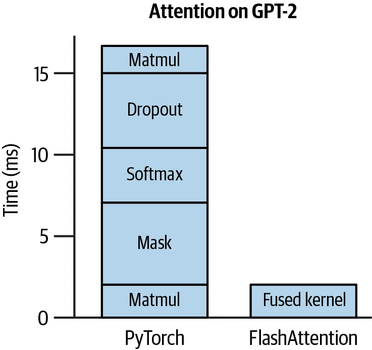Attention on GPT-2: FlashAttention fuses matmul, mask, softmax and dropout into one kernel

FlashAttention-2 reorganized work across warps and thread blocks to approach peak tensor-core throughput; FlashAttention-3 uses Hopper-specific features (asynchronous Tensor Memory Accelerator copies, warp specialization, FP8) to overlap data movement with computation. Separate decode-oriented kernels (FlashDecoding, split-KV kernels) parallelize over the KV sequence when there is only one query token. The point generalizes beyond attention: the kernel did not change the maths, only the schedule of memory accesses, and that alone moved attention from the bandwidth-bound region of the roofline toward the compute-bound one.

Model-level optimization: decoding, kernels and compilers

Where the previous section reduced the bytes each decode step must read, this one makes each read produce more tokens (decoding tricks) and makes the computation itself approach the roofline (kernels and compilers).

The autoregressive bottleneck

Decode produces one token per sequence per forward pass, and each pass reads the entire model. At batch size one the GPU is almost idle. The techniques in this section all try to get more than one token out of each expensive pass, either by guessing ahead and verifying, or by copying from the context.

Speculative decoding

Speculative decoding (Leviathan et al., 2023; Chen et al., 2023) pairs the target model you want outputs from with a cheap draft model. The draft proposes k tokens autoregressively (fast, because it is small). The target then processes all k proposals in one forward pass, exactly as it would process a k-token prompt, producing its own next-token distribution at every position. Each proposal is accepted or rejected by a rejection-sampling rule that compares the draft and target probabilities; the first rejected position is resampled from a corrected target distribution, and generation continues from there. The rule guarantees that the sequence of accepted tokens has exactly the distribution the target model alone would have produced. Output quality is unchanged by construction; only speed changes.

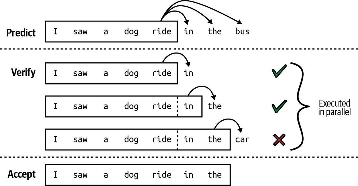Speculative decoding: a small draft model predicts several tokens, the target model verifies them in one pass and accepts the longest correct prefix

Why it helps: verifying k tokens costs the target one pass whose cost, in the bandwidth-bound regime, is barely more than a one-token pass (the weights are read once either way). If the draft's acceptance rate is high, you get several target-quality tokens per weight read. Speedups of 2 to 3× are typical when the draft agrees with the target on 70 to 90% of tokens, which it does for predictable text (code, boilerplate, restatements) and does less for creative or technical prose. Speculation gives back its gains at large batch sizes, when decode is already compute-bound and the extra verification FLOPs are no longer free.

Draft choices: a small model from the same family and tokenizer (a 1B or 7B draft for a 70B target); an n-gram lookup over the prompt itself (prompt-lookup decoding, free and effective for summarization and editing); the target's own early layers with an exit head (self-speculation, LayerSkip); or trained prediction heads (next section).

Parallel heads and lookahead

Medusa (Cai et al., 2024) removes the separate draft model by adding several lightweight decoding heads on top of the target's final hidden state, each trained to predict the token at position +2, +3 and so on. All heads fire in one pass and propose a tree of candidates, which tree attention verifies in a single additional pass with a custom mask; the longest accepted path is emitted. Heads are small (a layer or two), training is cheap (the backbone can stay frozen), and gains of 2 to 3× are reported. EAGLE improves on this by drafting from the hidden state with a small autoregressive head rather than independent heads, raising acceptance rates.

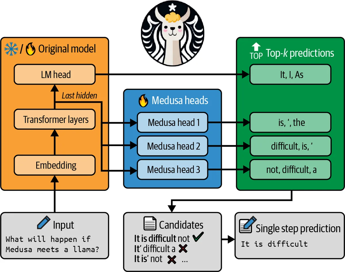Medusa adds extra decoding heads that each predict a later token; the candidates are verified in a single step

Lookahead decoding (Fu et al., 2024) needs no draft model or heads. It treats generating the next k tokens as solving a fixed-point system and applies Jacobi iteration: guess k tokens, run one parallel pass to refine all guesses, repeat until a prefix stabilizes, caching n-grams that appeared during iteration as future proposals. It trades extra FLOPs per step (which are free when bandwidth-bound) for fewer steps.

Inference with reference

When the output is likely to repeat spans of the input, as in summarization, question answering over a document, code editing and retrieval-augmented generation, the context itself is an excellent draft. Inference with reference (Yang et al., 2023) and prompt-lookup decoding match the last few generated tokens against the prompt and propose the span that followed them there; the target verifies as in speculative decoding. There is no second model, the method is exact, and on editing and RAG workloads the acceptance rate is high because the model is mostly copying.

Architectural changes

Some of the largest inference wins are decided at model design time. Mixture-of-experts models activate only a few expert feed-forward blocks per token, so a model with hundreds of billions of total parameters reads only a fraction of them per step; the cache for the inactive experts still occupies memory, but compute and (for the experts) bandwidth per token fall. Smaller dense models trained longer on more data (the trend from Chinchilla onwards) move quality into fewer parameters. State-space and hybrid architectures (Mamba and successors, hybrids such as Jamba) replace some attention layers with recurrent blocks whose state does not grow with sequence length, removing the KV cache for those layers. Application teams rarely choose these knobs, but they explain why newer models of the same quality are much cheaper to serve.

Kernels

A kernel is a function that runs on the accelerator. Every operator in a model (matmul, layer norm, softmax, activation, attention) becomes one or more kernels, and the quality of those kernels decides how much of the roofline you reach. Writing them well requires managing thread hierarchies, memory coalescing, shared-memory bank conflicts and occupancy, so most teams rely on vendor libraries (cuBLAS, cuDNN), engine-provided kernels, or Triton (a Python-based language that compiles to efficient GPU code and has made custom kernels far more accessible).

Four techniques recur in every fast kernel.

• Vectorization: load and operate on several contiguous elements per instruction (128-bit loads, SIMD math) so memory accesses are wide and few.
• Parallelization: split work across thousands of threads with minimal synchronization, and balance it so no streaming multiprocessor idles.
• Loop tiling: divide large matrices into tiles that fit in shared memory or registers, so each byte fetched from HBM is reused many times. FlashAttention is tiling applied to attention; cuBLAS matmuls are tiling applied to GEMM.
• Operator fusion: combine consecutive operators (matmul, bias, activation; or the whole attention block) into one kernel so intermediates stay in registers and SRAM instead of round-tripping to HBM. Fusion attacks memory traffic directly and also removes kernel-launch overhead, which matters at batch size one where each launch is a few microseconds and a decode step launches hundreds of kernels.

Compilers

AI compilers take a model graph and generate fused, tuned kernels automatically. torch.compile (PyTorch 2) captures the graph with TorchDynamo and generates Triton kernels with TorchInductor; for LLM decode it also enables CUDA graphs, which replay a whole step's kernel launches with one call and remove most launch overhead. XLA compiles JAX and TensorFlow graphs for TPUs and GPUs with aggressive whole-program fusion. TensorRT and TensorRT-LLM are NVIDIA's inference compilers and runtime, with calibrated quantization, fused attention, in-flight batching and the best absolute numbers on NVIDIA hardware at the cost of an explicit build step per model and shape. Apache TVM and MLIR-based stacks target heterogeneous hardware with auto-tuned schedules. For most teams the practical choice is which serving engine to adopt, since each embeds a compiler strategy.

The PyTorch case study

The PyTorch team's "GPT, fast" write-up showed how model-level techniques compound on Llama 7B decoding on a single A100, in under a thousand lines of native PyTorch.

Step	Technique	Approximate tokens per second
Baseline	Eager PyTorch	~25
+ torch.compile	Fused kernels, static KV cache, CUDA graphs	~105
+ INT8 weight-only quantization	Half the bytes per step	~155
+ INT4 weight-only quantization (GPTQ)	Quarter of the bytes per step	~200
+ Speculative decoding	Several tokens per target pass	~240

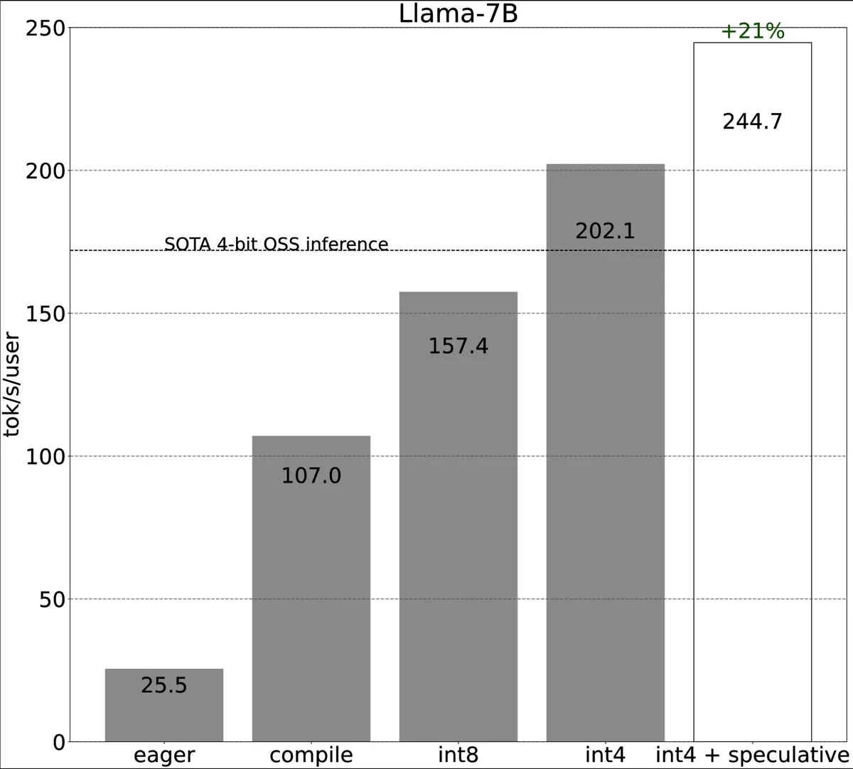Llama 7B tokens per second per user with successive optimizations: compilation, int8, int4 and speculative decoding

Each step attacks a different limit. Compilation removes overhead (launch latency and unfused memory traffic) that had the GPU idle most of the time. Quantization reduces the bytes read per step, which is the real bound once overhead is gone. Speculative decoding amortizes each weight read over several tokens. They are complementary because they are not fighting over the same bottleneck. The order also matters: quantization before compilation would have shown little, since the system was overhead-bound, not bandwidth-bound, until compilation fixed it.

Service-level optimization

Service-level techniques leave the model untouched and change how requests are scheduled onto hardware. They never change output quality, which makes them the safest optimizations to adopt, and because a single decode stream uses so little of a GPU, they are also where the largest throughput gains live.

Batching

Batching runs several sequences through the model per step so that the weights, read once from HBM, serve many tokens. Three schemes exist.

Static batching collects a fixed number of requests, runs them together, and returns when the whole batch finishes. Early arrivals wait for late ones, and once the batch starts every slot is held until the longest sequence finishes, so a 10-token answer occupies a slot for the 500 steps of its neighbour.

Dynamic batching adds a timer: dispatch when the batch is full or when a time window (tens of milliseconds) expires. It bounds queueing latency and is the standard for non-autoregressive models (embeddings, classifiers), but it still wastes the slots of early finishers in generation.

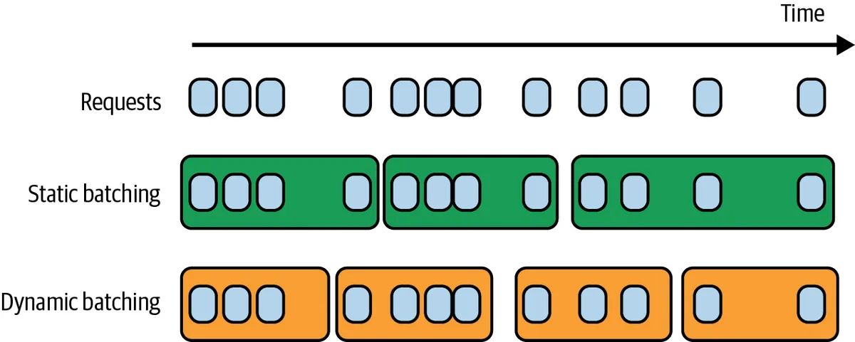Static batching waits for a full batch; dynamic batching also dispatches when a time window expires, keeping latency manageable

Continuous batching (also called in-flight batching; introduced as iteration-level scheduling in Orca, Yu et al., 2022) reschedules at every decode step. When a sequence emits its stop token its slot is freed immediately and a waiting request is admitted, usually by running its prefill and then joining the decode batch. The GPU stays full, no request waits for strangers to finish, and throughput gains over static batching range from 2× to over 10× depending on how variable output lengths are. The engineering requirements are a scheduler that reasons per step and a KV cache that can grow and shrink per sequence without fragmentation, which is why PagedAttention and continuous batching arrived together in vLLM.

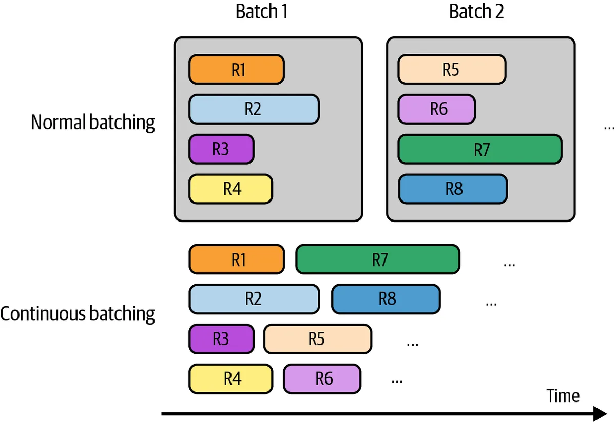Continuous batching returns each finished response immediately and slots a new request into its place

Continuous batching exposes one tension: when a new request's prefill is run inside a decode batch, every other sequence's step takes as long as that prefill, which spikes their TPOT. Engines mitigate with chunked prefill (splitting a long prompt's prefill across several steps so each step's cost is bounded) and with scheduling policies that prioritize TTFT or TPOT according to the SLO.

Scheme	Wait before start	Slot utilization	Complexity	Use
Static	Until batch fills	Poor with variable lengths	Trivial	Offline batch jobs
Dynamic	Until full or timer	Poor for generation	Low	Embedding, classification, fixed-length outputs
Continuous	None beyond prefill scheduling	High	High (engine-provided)	All LLM serving

Decoupling prefill and decode

Prefill and decode want different hardware behaviour: prefill is compute-bound and benefits from batching tokens, decode is bandwidth-bound and benefits from batching sequences, and mixing them on one GPU makes each interfere with the other's latency. Disaggregated serving (DistServe, Splitwise, and the production designs that followed) runs prefill on one pool of GPUs and decode on another, transferring each request's KV cache from a prefill worker to a decode worker over NVLink or the network once its first token is produced.

The benefits are independent scaling (add prefill capacity when prompts get longer, decode capacity when outputs do), isolation (a burst of long prompts no longer stalls everyone's token stream), per-phase tuning (batch sizes, parallelism degree and even chip type can differ), and the option of heterogeneous hardware (compute-rich chips for prefill, bandwidth-rich for decode). The cost is moving the KV cache, hundreds of megabytes to gigabytes per long request, which is why disaggregation needs fast interconnect and is a large-scale technique. DistServe reported serving up to several times more requests within the same latency SLO than colocated serving, a goodput win rather than a raw throughput win.

Prompt caching

Many requests share a prefix: the same system prompt, the same few-shot examples, the same long document being asked different questions, or the same conversation history extended by one turn. Prompt caching (prefix caching) keeps the KV cache for a prefix after its first computation and reuses it for later requests that start with the same tokens, so only the unique suffix is prefilled. Since prefill cost is linear in prompt length and dominates TTFT, the savings for long shared prefixes are large.

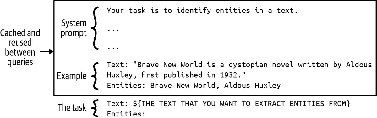A prompt cache stores the system prompt and examples shared across queries so only the task-specific part is processed each time

Implementation choices: automatic engines (vLLM's prefix caching, SGLang's RadixAttention) hash or trie-index cached blocks and match any request's longest cached prefix transparently; explicit APIs ask the developer to mark cache breakpoints. Eviction is usually LRU over cached blocks, and the cache lives in GPU memory (competing with live KV cache) or is tiered to host memory. Because the cache is keyed on exact token prefixes, caching only works if the shared part comes first and is byte-identical: put the static system prompt and examples at the start and the per-request content at the end, and avoid injecting timestamps or user IDs before the static portion.

Hosted providers expose this as pricing. At the time of writing, Anthropic charges about 1.25× the input price to write a cache and 0.1× to read it, with the book quoting savings of up to 90% on cost and 75% on latency for long cached prefixes; Google's context caching and OpenAI's automatic prompt caching (a 50% discount on cached input tokens) are the same mechanism with different terms. Three scenarios dominate: long system prompts and tool definitions reused on every call, many-shot prompts whose examples are the bulk of the tokens, and multi-turn conversations where each turn re-sends the whole history.

Parallelism

When one accelerator is not enough, work is split across several. The strategies differ in what they split and what they must communicate.

Replica (data) parallelism runs full copies of the model on separate devices behind a load balancer. It scales throughput linearly with no inter-device communication and is the default whenever the model fits on one device (or one tensor-parallel group). Autoscaling adjusts the replica count with traffic.

Tensor parallelism splits individual weight matrices across devices: each holds a shard of every layer, computes a partial result, and an all-reduce (or all-gather) combines them, twice per transformer layer. It lowers per-request latency because every matmul is shared across devices, and it is how 70B and larger models fit at all. The communication is frequent and large, so it is confined to devices on fast interconnect: within a node over NVLink (about 900 GB/s per H100), not across nodes over InfiniBand.

Pipeline parallelism assigns consecutive layers to consecutive devices; activations flow from stage to stage once per forward pass, so communication is small and tolerates slower links. Its cost is pipeline bubbles: with one request in flight only one stage works at a time. Micro-batching keeps several micro-batches moving through the stages at once so most devices stay busy, at the price of latency for each individual request.

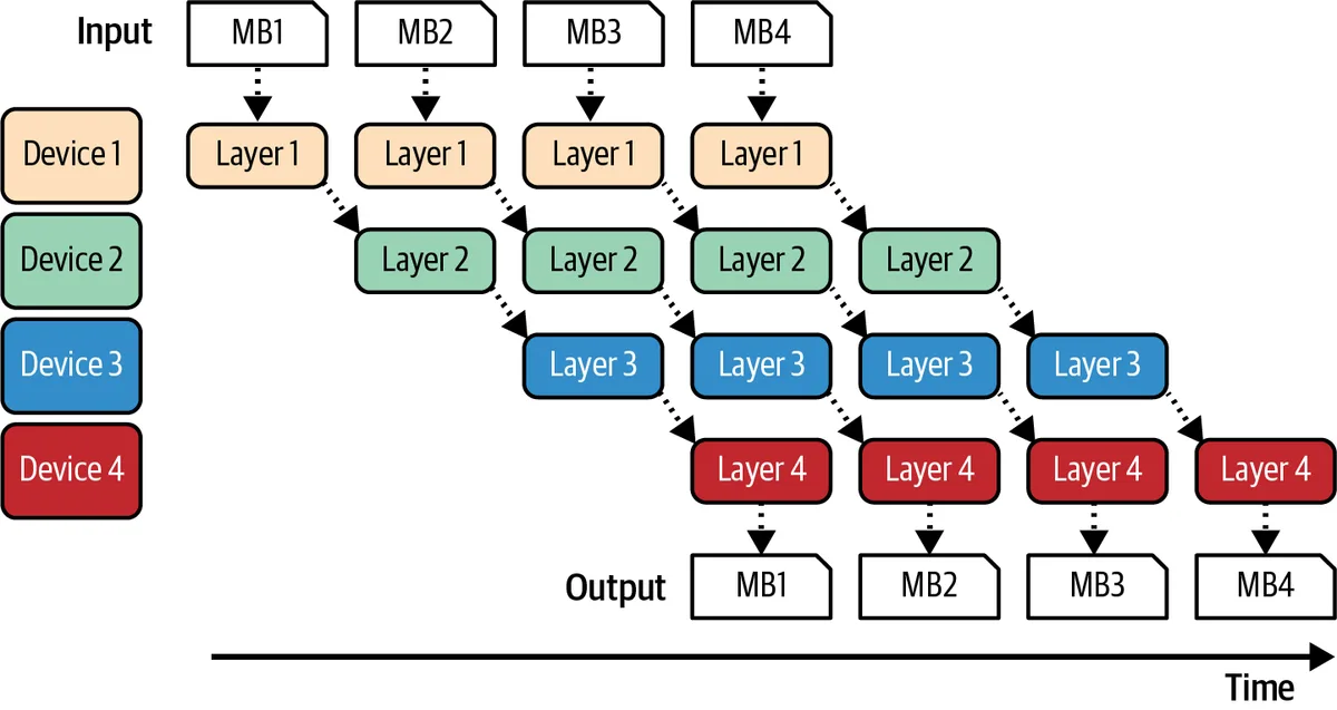Pipeline parallelism: each device holds some layers, and micro-batches flow through them so the devices work concurrently

Context (sequence) parallelism splits a single very long sequence across devices along the token dimension. Attention requires every token to see every other, so keys and values are passed around the devices in a ring (ring attention) while each computes attention for its own chunk, overlapping communication with computation. It is what makes million-token contexts feasible and is also used to spread a single request's enormous KV cache across devices. Expert parallelism places different MoE experts on different devices and routes tokens to them, a natural fit for mixture-of-experts models.

Strategy	Splits	Communication	Best for	Limit
Replica	Nothing (copies)	None	Throughput when the model fits	Memory per replica
Tensor	Each weight matrix	Per layer, large, needs NVLink	Fitting big models, lowering latency	Node boundary
Pipeline	Layers	Per stage, small	Spanning nodes with modest links	Bubbles; latency
Context / sequence	Tokens of one sequence	Ring exchange of K and V	Very long contexts	Attention communication
Expert	MoE experts	All-to-all token routing	Mixture-of-experts models	Load imbalance

Production systems combine them: tensor parallelism within a node, pipeline parallelism across nodes if the model still does not fit, replicas of that whole arrangement for throughput, and context parallelism only for extreme sequence lengths. Tensor parallelism is preferred for latency, pipeline for bandwidth-efficient capacity, replicas for everything else.

Design trade-offs

Which optimization for which problem

Symptom	Likely bound	First moves	Then
High TTFT on long prompts	Prefill compute, queueing	Prompt caching for shared prefixes, shorter prompts, chunked prefill	More compute, disaggregated prefill pool, tensor parallelism
High TPOT at low concurrency	Decode bandwidth	Weight quantization (INT8, then INT4), KV cache quantization, compilation	Speculative or Medusa decoding, higher-bandwidth hardware
Low throughput, GPU underutilized	Scheduling	Continuous batching with a paged KV cache	Larger batch, replica parallelism
Out of memory as concurrency grows	KV cache capacity	PagedAttention, GQA model, KV quantization, shorter contexts	More memory per device, tensor parallelism, disaggregation
Model does not fit on one GPU	Capacity	INT4 or FP8 weights	Tensor parallelism within node, pipeline across nodes
p99 latency far above p50	Interference, tail inputs	Separate prefill from decode scheduling, cap max tokens, priority queues	Disaggregated serving
Cost too high for offline workloads	Pricing model	Batch API or offline batch job at maximum batch size	Smaller or distilled model

Quality impact and who can apply each technique

Technique	Changes outputs?	Applied by	Main metric improved
Weight quantization	Yes (small, must evaluate)	Self-hosters, providers	TPOT, memory, cost
Pruning	Yes	Model owners	Memory, compute
Distillation	Yes (new model)	Model owners	Everything, at a quality ceiling
MQA / GQA / windowed / cross-layer attention	Yes (training-time)	Model trainers	KV memory, TPOT
PagedAttention	No	Serving engine	Throughput, concurrency
FlashAttention and fused kernels	No	Serving engine, compilers	Prefill speed, memory
Speculative decoding, lookahead, reference	No (exact)	Serving engine	TPOT at low batch
Medusa / EAGLE heads	No at verification; needs trained heads	Model owners with engine support	TPOT
Continuous batching	No	Serving engine	Throughput, goodput
Prompt caching	No	Serving engine, API users via prompt layout	TTFT, cost
Prefill/decode disaggregation	No	Large-scale operators	Goodput, tail latency
Parallelism	No	Self-hosters, providers	Capacity, latency or throughput by type
Batch API, streaming, shorter prompts and outputs	No	API users	Cost, perceived latency

Interview angle

• Why is LLM decoding memory-bandwidth-bound, and what follows from that? Each decode step reads every weight (and the KV cache) from HBM to produce one token per sequence, so FLOPs per byte are tiny and the chip waits on memory. Consequences: tokens per second at batch one is roughly bandwidth divided by bytes per step, quantization speeds decode almost linearly, batching is nearly free until the batch is large, and extra FLOPs (speculation, lookahead) cost little. Prefill, which processes all prompt tokens at once, is compute-bound and behaves differently.

• Define TTFT, TPOT and goodput. Why not just report average latency and tokens per second? TTFT is request to first token (queueing plus prefill); TPOT is the mean gap between later tokens (decode); total latency is TTFT plus TPOT times output tokens. Goodput is requests per second that meet the latency SLO. Averages hide the tail that users feel, and raw throughput can be raised by batching so hard that most requests violate the SLO; goodput ties capacity to the promise you made.

• Estimate the KV cache for Llama 2 70B serving 64 users at 8k context. Per token: 2 × 80 layers × 8 KV heads × 128 × 2 bytes ≈ 320 KB. Per sequence at 8,192 tokens: ≈ 2.7 GB. For 64 sequences: ≈ 172 GB, more than the model's own 140 GB of BF16 weights. So you would need several 80 GB GPUs for cache alone, or KV quantization, shorter contexts, or a model with fewer KV heads; and PagedAttention to avoid wasting what you have.

• Explain speculative decoding and why it does not change the model's output distribution. A cheap draft proposes k tokens; the target scores them in one pass; a rejection-sampling rule accepts each draft token with probability min(1, p_target / p_draft) and resamples from the adjusted target distribution at the first rejection. Because the acceptance rule is constructed to make accepted tokens follow the target's distribution exactly, outputs are statistically identical; speed improves by the expected number of accepted tokens per target pass, which depends on draft agreement.

• What does PagedAttention fix? Engines used to reserve a contiguous KV region per request sized for the maximum length, wasting memory to internal and external fragmentation and limiting batch size. PagedAttention stores KV in fixed-size blocks mapped by a per-sequence block table, allocated on demand and shareable across sequences with copy-on-write, cutting waste to a few percent and allowing far more concurrent sequences, which continuous batching turns into throughput.

• Compare static, dynamic and continuous batching for a chat service. Static waits for a full batch and holds every slot until the longest response ends, so short answers waste capacity and early arrivals wait. Dynamic adds a timeout, fixing the wait but not the wasted slots. Continuous batching reschedules every decode step: finished sequences leave, new ones join, the GPU stays full; it needs a per-step scheduler and a paged KV cache and is the default in modern engines. Watch for prefill of new arrivals spiking TPOT; chunked prefill mitigates it.

• You can choose between a chip with 2× the FLOP/s and one with 2× the memory bandwidth for a chatbot. Which? For typical chat (short prompts, long outputs, moderate concurrency) decode dominates and is bandwidth-bound, so the bandwidth chip gives more tokens per second per user. The FLOP/s chip wins for long-prompt, high-concurrency or offline batch workloads that are compute-bound. Decide by profiling arithmetic intensity against the roofline, and check memory capacity for KV cache first either way.

• How would you lay out a prompt to maximize prompt-cache hits, and what does it save? Put the static content first (system prompt, tool schemas, few-shot examples, the shared document) and the per-request content last; keep the static part byte-identical (no timestamps or per-user fields before it). Caching skips prefill for the matched prefix, cutting TTFT and input cost; providers price cache reads at about a tenth of normal input tokens, so for long prefixes the savings approach 90% on that portion.

• When is tensor parallelism the wrong choice? Across nodes: it synchronizes twice per layer with large transfers and needs NVLink-class bandwidth, so over InfiniBand or Ethernet it stalls. Use pipeline parallelism across nodes (small activations once per stage, at the cost of bubbles) and tensor parallelism only within a node. If the model already fits on one device, use replicas instead, since they need no communication at all.

Pitfalls and misconceptions

• Judging hardware by peak FLOP/s. Decode is bandwidth-bound for most interactive workloads; a chip with more bandwidth and memory beats one with more FLOP/s. Vendor FLOP/s headlines also often assume 2:4 sparsity; halve them for dense models.
• Reporting average latency. Tails dominate user experience. Report p50, p90 and p99 TTFT and TPOT with input and output lengths, under realistic concurrency.
• Expecting quantization to be free everywhere. INT8 weight-only usually is; INT4 costs measurable quality, especially on small models and on specific capabilities. Evaluate the exact artefact you serve, and remember that different providers' versions of "the same" open model differ for this reason.
• Confusing low MFU with bad engineering. In decode, low MFU is structural. Look at MBU; if it is high, the stack is efficient and only fewer bytes or more bandwidth will help.
• Assuming speculative decoding helps at any batch size. Its gains come from spare compute during bandwidth-bound decode. At large batch, decode is compute-bound and verification FLOPs are no longer free; gains shrink or reverse.
• Breaking prompt-cache prefixes. A timestamp, request ID or user name placed before the static system prompt invalidates the shared prefix on every call. Static first, dynamic last, byte-identical.
• Implementing batching yourself. Continuous batching with a paged KV cache is subtle; vLLM, TensorRT-LLM, TGI and SGLang have it built in. Spend effort on evaluation and prompt layout instead.
• Forgetting the KV cache in capacity planning. Weights are fixed; the cache grows with context and concurrency and is what runs out first. Budget it explicitly and monitor it.

Key terms

Term	Meaning
Prefill	The phase that processes all prompt tokens in parallel, writes the KV cache and produces the first token; compute-bound
Decode	The phase that generates one token per sequence per forward pass; memory-bandwidth-bound at small batch
Arithmetic intensity	FLOPs performed per byte moved from memory; compared against the hardware's ops:byte ratio
Roofline model	A chart of attainable FLOP/s against arithmetic intensity with a bandwidth-sloped roof and a flat compute roof
TTFT / TPOT	Time to first token; time per output token
Goodput	Requests (or tokens) per second that meet the latency SLO
MFU / MBU	Model FLOP/s utilization; model bandwidth utilization, each as a fraction of hardware peak
HBM / SRAM	High-bandwidth device memory holding weights and cache; small on-chip memory where kernel tiles live
Tensor core	A GPU unit performing small dense matrix multiply-accumulates per instruction at reduced precision
KV cache	Stored keys and values of earlier tokens at every layer, making decode linear rather than quadratic
MQA / GQA	Multi-query and grouped-query attention: query heads share one or a few KV heads to shrink the cache
Sliding-window attention	Each token attends only to the previous w tokens, bounding cache and compute on those layers
Cross-layer attention	Adjacent layers share one KV cache
PagedAttention	Block-based KV cache allocation with per-sequence block tables, removing fragmentation and enabling sharing
FlashAttention	An IO-aware, tiled, exact attention kernel that never materializes the n × n score matrix in HBM
Operator fusion	Combining several operators into one kernel so intermediates stay on chip
Speculative decoding	A draft proposes several tokens, the target verifies them in one pass with a rejection rule that preserves its output distribution
Acceptance rate	The fraction of draft tokens the target accepts; determines speculative speedup
Medusa heads / tree attention	Extra prediction heads proposing a tree of future tokens, verified in one masked pass
Lookahead (Jacobi) decoding	Iteratively refining several guessed tokens in parallel until a prefix converges
Inference with reference	Drafting from spans of the prompt itself when outputs copy the input
Continuous (in-flight) batching	Rescheduling the batch at every decode step so finished sequences leave and new ones join
Chunked prefill	Splitting a long prompt's prefill across several steps to bound interference with decoding sequences
Prefill/decode disaggregation	Running the two phases on separate GPU pools and transferring the KV cache between them
Prompt (prefix) caching	Reusing the KV cache of a shared prompt prefix across requests
Tensor / pipeline / replica / context parallelism	Splitting matrices, layers, whole copies, or the token sequence across devices
Pipeline bubble	Idle time in pipeline parallelism while stages wait for each other

Further reading

• AI Engineering, Chapter 9 (Inference Optimization); companion material at https://github.com/chiphuyen/aie-book
• Kwon et al., "Efficient Memory Management for Large Language Model Serving with PagedAttention" (vLLM, 2023): https://arxiv.org/abs/2309.06180
• Dao et al., "FlashAttention: Fast and Memory-Efficient Exact Attention with IO-Awareness" (2022): https://arxiv.org/abs/2205.14135
• Dao, "FlashAttention-2: Faster Attention with Better Parallelism and Work Partitioning" (2023): https://arxiv.org/abs/2307.08691
• Leviathan, Kalman and Matias, "Fast Inference from Transformers via Speculative Decoding" (2023): https://arxiv.org/abs/2211.17192
• Chen et al., "Accelerating Large Language Model Decoding with Speculative Sampling" (2023): https://arxiv.org/abs/2302.01318
• Cai et al., "Medusa: Simple LLM Inference Acceleration Framework with Multiple Decoding Heads" (2024): https://arxiv.org/abs/2401.10774
• Fu et al., "Break the Sequential Dependency of LLM Inference Using Lookahead Decoding" (2024): https://arxiv.org/abs/2402.02057
• Yang et al., "Inference with Reference: Lossless Acceleration of Large Language Models" (2023): https://arxiv.org/abs/2304.04487
• Shazeer, "Fast Transformer Decoding: One Write-Head is All You Need" (MQA, 2019): https://arxiv.org/abs/1911.02150
• Ainslie et al., "GQA: Training Generalized Multi-Query Transformer Models from Multi-Head Checkpoints" (2023): https://arxiv.org/abs/2305.13245
• Brandon et al., "Reducing Transformer Key-Value Cache Size with Cross-Layer Attention" (2024): https://arxiv.org/abs/2405.12981
• Yu et al., "Orca: A Distributed Serving System for Transformer-Based Generative Models" (OSDI 2022): https://www.usenix.org/conference/osdi22/presentation/yu
• Zhong et al., "DistServe: Disaggregating Prefill and Decoding for Goodput-optimized Large Language Model Serving" (2024): https://arxiv.org/abs/2401.09670
• Williams, Waterman and Patterson, "Roofline: An Insightful Visual Performance Model for Multicore Architectures" (CACM 2009)
• Frantar et al., "GPTQ: Accurate Post-Training Quantization for Generative Pre-trained Transformers" (2022): https://arxiv.org/abs/2210.17323
• Lin et al., "AWQ: Activation-aware Weight Quantization for LLM Compression and Acceleration" (2023): https://arxiv.org/abs/2306.00978
• Xiao et al., "Efficient Streaming Language Models with Attention Sinks" (2023): https://arxiv.org/abs/2309.17453
• PyTorch team, "Accelerating Generative AI with PyTorch II: GPT, Fast" (2023): https://pytorch.org/blog/accelerating-generative-ai-2/
• Character.AI, "Optimizing AI Inference at Character.AI" (2024 engineering blog post)