You will probably never pre-train a foundation model, but every decision you make on top of one depends on how it was built. Chapter 2 follows a model from its training data through its architecture and size, into post-training (where a text completer becomes an assistant), and finally to sampling, the step that turns a probability distribution into the text you see. The chapter ends with the two behaviors that make AI engineering hard: outputs are inconsistent, and models hallucinate.

For an engineer this is the diagnostic vocabulary. When a model is weak in Hindi, that is a training-data question. When long prompts are slow and expensive, that is attention and the KV cache. When JSON comes back malformed, that is a sampling question. When a model confidently invents a citation, there are two competing explanations and each suggests different mitigations.

In one minute

• Models learn what their data contains. Common Crawl-derived corpora are roughly half English, dominated by general web content, and thin on specialized domains, so models are weaker on low-resource languages and niche fields and cost more tokens per sentence outside English.
• The transformer replaced the seq2seq RNN bottleneck with attention: each token builds a query, compares it to every earlier token's key, and sums their values. Keys and values are cached (the KV cache), which is why inference splits into a parallel prefill phase and a sequential decode phase.
• Model size has three axes: parameters, training tokens and FLOPs (roughly 6 × parameters × tokens). Chinchilla says a compute-optimal model needs about 20 tokens per parameter; production models train far past that because inference cost matters more than training cost.
• Scaling is bounded by data (public high-quality text runs out this decade) and electricity (data centers already use 1 to 2 percent of global power).
• Post-training has two steps: SFT on (prompt, response) demonstrations teaches the conversation format; preference finetuning (RLHF with a reward model and PPO, or DPO directly on preference pairs, or RLAIF with AI feedback) pushes outputs toward what people prefer.
• Sampling picks the next token from the softmax distribution. Temperature reshapes the distribution; top-k and top-p truncate it; stopping conditions end generation. More samples plus a selector (best-of-N, majority vote) buys quality with test-time compute.
• Structured outputs come from prompting, post-processing, constrained sampling (mask invalid tokens with a grammar) or finetuning, in increasing order of reliability and cost.
• Models are probabilistic. Inconsistency means the same prompt yields different answers; hallucination means fluent fabrication. The two leading explanations are self-delusion (the model cannot tell its own tokens from given facts) and mismatched internal knowledge (post-training taught it to answer beyond what it knows).

Training data

What the internet actually contains

A model can only learn patterns present in its data. The largest public source is Common Crawl, a nonprofit that crawls two to three billion web pages each month. Google's C4 (Colossal Clean Crawled Corpus) is a cleaned Common Crawl snapshot; The Pile, RefinedWeb and FineWeb are other filtered derivatives. Crawled data is big, cheap and indiscriminate: peer-reviewed papers sit next to spam, clickbait, propaganda and, increasingly, machine-generated text.

Three properties of this data shape every model trained on it.

• Language skew. English is roughly 46 percent of Common Crawl; the next largest languages (Russian, German, Chinese, Japanese, French, Spanish) each sit around 4 to 6 percent, and most of the world's languages are a rounding error. Some languages with tens of millions of speakers (Punjabi, Swahili) have a smaller share than their speaker count would predict by an order of magnitude.
• Domain skew. Topic categories in C4 are dominated by general web content such as business, entertainment and technology. Chemistry, medicine, law and the long tail of professional knowledge are thin, often paywalled, or sit in formats (PDF tables, lab notebooks) that crawlers handle badly.
• Quality variance and legal exposure. Scraped data contains copyrighted material and personal information collected without consent. Those issues are unresolved and are the root of several ongoing lawsuits and of publishers blocking crawlers.

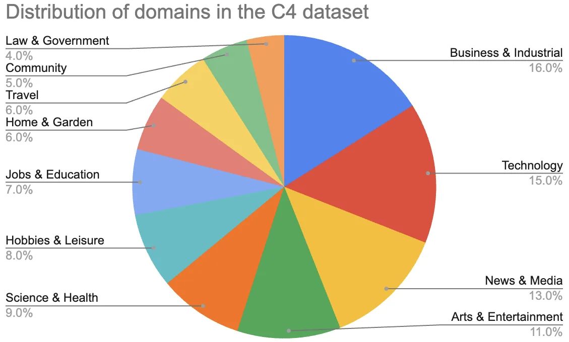Figure 2-3. Distribution of domains in the C4 dataset

Multilingual data

Language skew shows up directly in benchmarks. GPT-4 scores higher on MMLU in English than in any other language, and the gap on math problems is larger still, because reasoning in a low-resource language compounds weaker language modeling with weaker task knowledge.

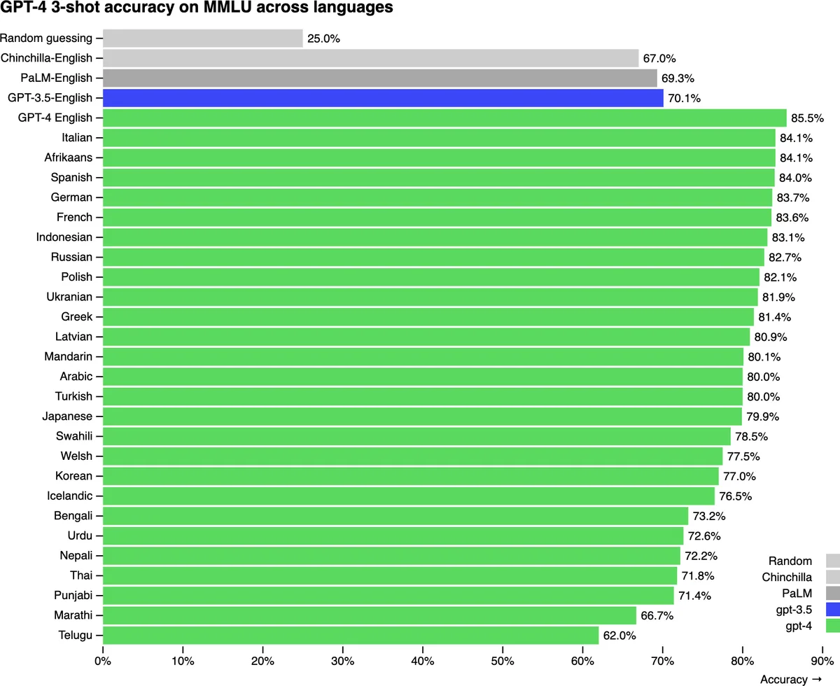Figure 2-1. On the MMLU benchmark, GPT-4 performs better in English than in any other language

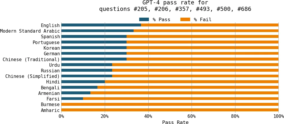Figure 2-2. GPT-4 is much better at math in English than in other languages

Tokenization makes it worse in two ways. Tokenizers are trained on the same skewed data, so a sentence in Hindi or Burmese fragments into many more tokens than its English equivalent (on the MASSIVE dataset, median token counts for the same sentences ran roughly four times higher in Hindi and ten times higher in Burmese than in English). That means higher cost per request, less effective context, and higher latency, since decode time scales with output tokens. Translating to English first is a common workaround but loses nuance and introduces its own errors.

Domain-specific data

General models do well on domains well represented online and poorly elsewhere. Protein structure, drug discovery, legal discovery and medical imaging all needed either domain-specific pre-training (AlphaFold, NVIDIA's BioNeMo, BloombergGPT on financial text) or domain finetuning on top of a general model (Med-PaLM 2). When your use case lives in a thin domain, expect to supply the data yourself through retrieval or finetuning, and expect benchmarks that look fine on general knowledge to say little about your task.

Quality over quantity

Scaling data indiscriminately stopped being the whole story around 2023. Microsoft's Phi series showed that small models trained on curated "textbook quality" data outperform larger models trained on raw web text on reasoning benchmarks, and many labs now spend as much effort filtering data as collecting it. Typical pipeline stages:

Stage	What it does	Why it matters
Heuristic filters	Drop documents by length, symbol ratio, boilerplate markers, bad-word lists	Cheap removal of obvious junk
Deduplication	Remove exact and near-duplicate documents (MinHash, suffix arrays)	Duplicates cause memorization and waste compute
Perplexity or classifier filters	Score text with a reference model or quality classifier; keep the good tail	Approximates "would a careful human want this in the corpus"
Domain mixing	Choose proportions of web, books, code, papers, dialogue	Composition drives capability profile: more code improves structured reasoning even off code
Decontamination	Remove benchmark test sets from training data	Otherwise evaluation scores are memorization, not capability

Chapter 8 returns to this pipeline from the application side, where the same tools (dedup, filtering, mixing) apply to finetuning data.

Modeling: the transformer

Why the transformer replaced seq2seq

Before 2017 the dominant architecture for text-to-text tasks was seq2seq: an RNN encoder read the input token by token into a hidden state, and an RNN decoder generated the output from that state. It had two problems. The final hidden state was a bottleneck: everything about a long input had to fit through one vector. And the computation was sequential: token t could not be processed until token t−1 was, so training could not use parallel hardware well.

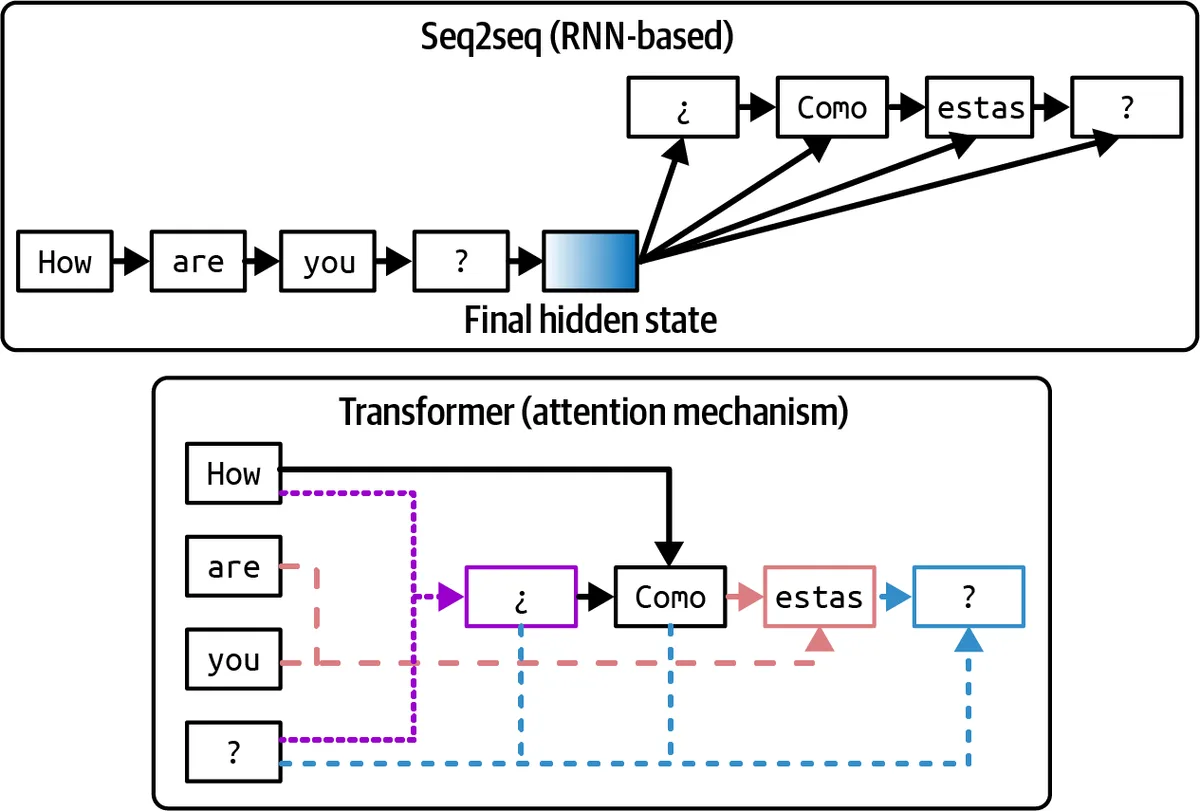A seq2seq RNN reads the input through a bottleneck state, while a transformer attends to every input token directly

The transformer (Vaswani et al., 2017) fixed both. Attention lets the decoder look at every input token directly instead of through the bottleneck, and because attention has no recurrence, all input tokens are processed in parallel. Output generation is still sequential (each token conditions on the previous one), which is why inference has two phases:

• Prefill: all prompt tokens are processed in parallel and their keys and values are computed. This is compute-bound and determines time to first token.
• Decode: output tokens are generated one at a time, each attending to everything before it. This is memory-bandwidth-bound and determines time per output token.

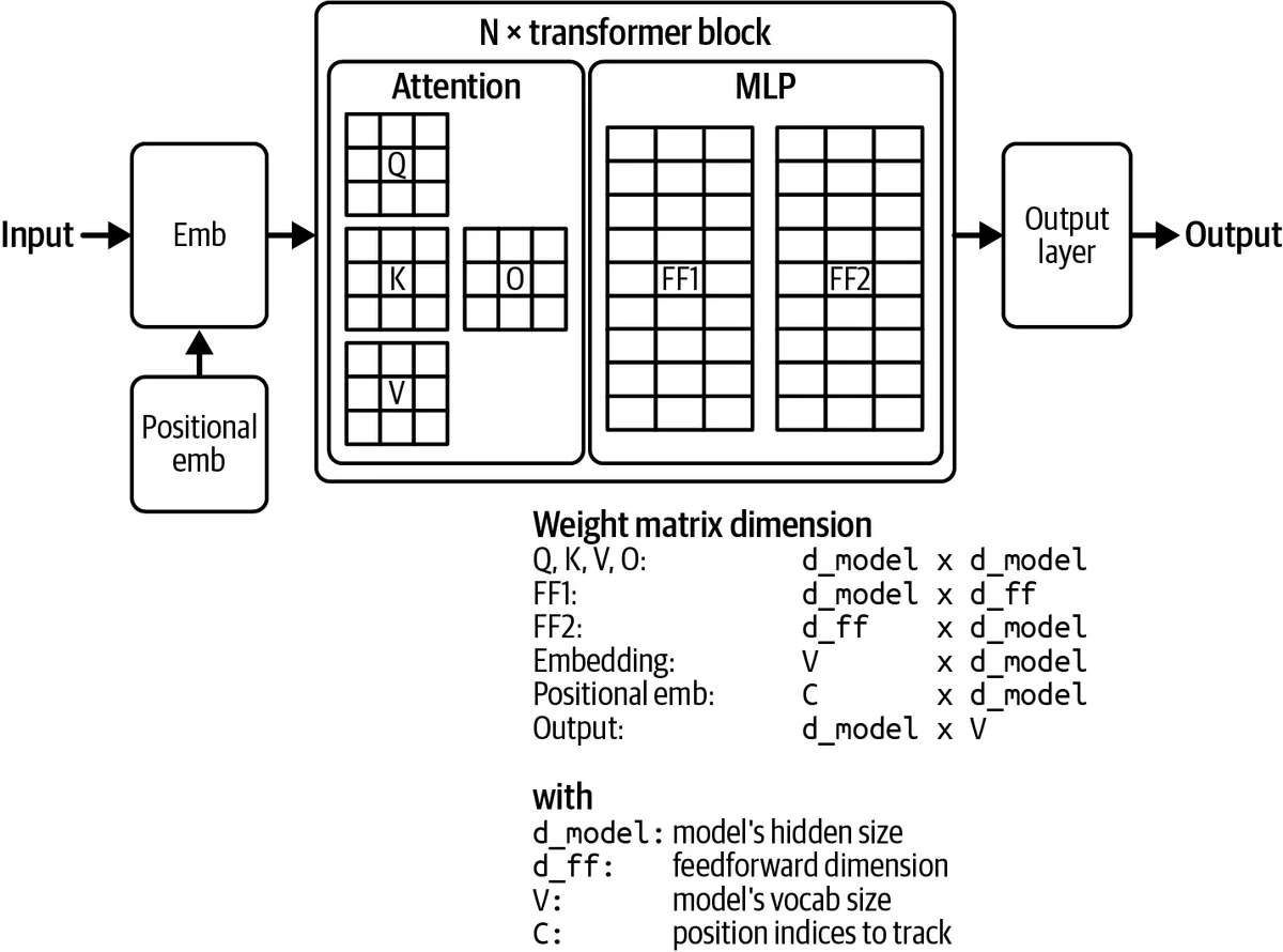Figure 2-6. Transformer model architecture

Attention, keys, values and the KV cache

For each token the model computes three vectors through learned projection matrices:

• a query (Q): what this token is looking for,
• a key (K): what this token offers to be matched against,
• a value (V): the content this token contributes if attended to.

The attention output for a token is a weighted sum of all values, with weights from the softmax of its query dotted with every key, scaled by the square root of the key dimension to keep the softmax from saturating:

Attention(Q, K, V) = softmax(Q · K^T / sqrt(d_k)) · V

The intuition is a soft dictionary lookup: instead of returning the one value whose key matches exactly, you return a blend of all values weighted by how well their keys match. In a decoder, a causal mask prevents a token from attending to later tokens, which is what makes next-token prediction well defined.

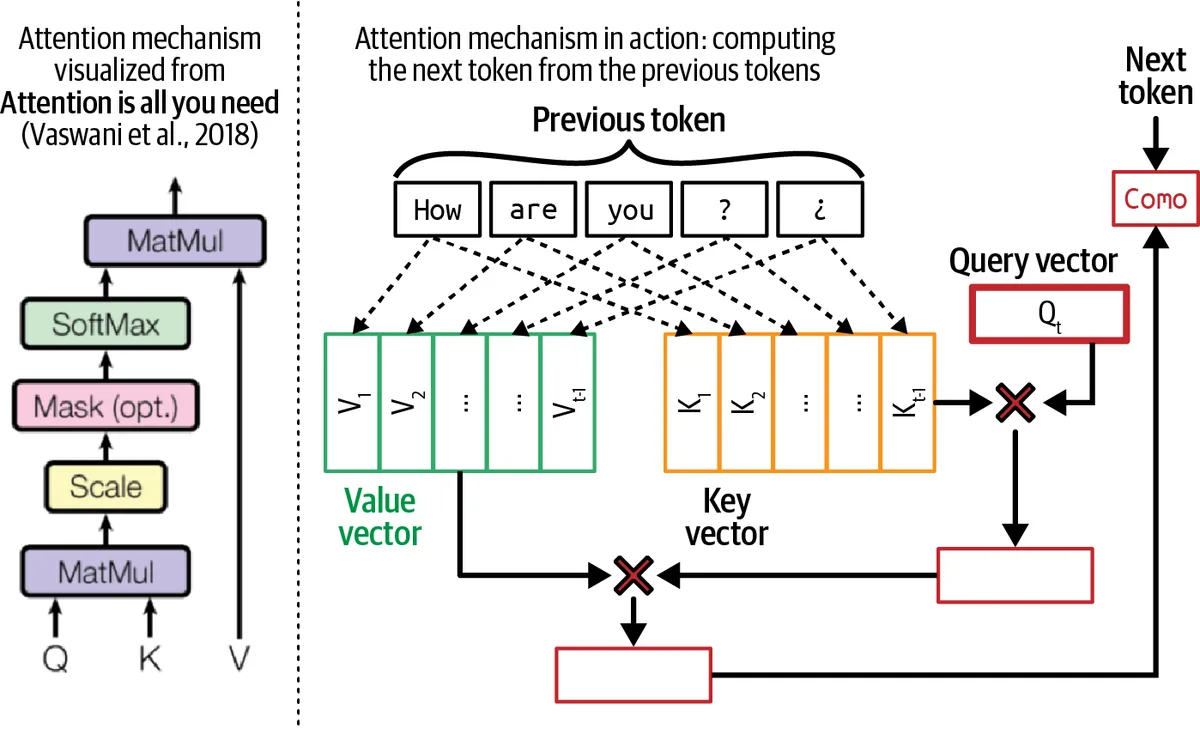Figure 2-5. An example of the attention mechanism in action

Two consequences matter for engineering. First, every earlier token's key and value are needed at every decode step, so they are stored in the KV cache. The cache grows linearly with context length and is a large share of GPU memory at long contexts, which is why long-context inference is expensive and why Chapter 9 spends time on it. Second, computing attention over n tokens costs on the order of n² in the naive implementation, which drove optimizations such as FlashAttention and architectural variants that share keys and values across heads (multi-query and grouped-query attention, used in Llama 2 70B and Llama 3).

Multi-head attention runs several attention computations in parallel with different projections, so different heads can track different relations (syntax, coreference, position). Llama 2 7B uses 32 heads; the 70B model uses 64. Outputs of all heads are concatenated and projected back to the model dimension.

Inside a transformer block

A transformer is a stack of identical blocks, each containing an attention module and a position-wise feed-forward network (MLP), with residual connections and layer normalization around both. Attention moves information between positions; the MLP transforms each position independently and holds much of the model's factual "knowledge". Before the blocks sits an embedding module (token embeddings plus positional information) and after them an output layer (sometimes called the unembedding) that projects the final hidden state onto the vocabulary to produce logits.

Llama 2 variant	Blocks (layers)	Model dimension	Attention heads	Vocabulary
7B	32	4,096	32	32,000
13B	40	5,120	40	32,000
70B	80	8,192	64 (grouped-query)	32,000

Encoder, decoder and encoder-decoder

The original transformer had an encoder and a decoder. Later models kept one or the other.

Feature	Encoder-only	Decoder-only	Encoder-decoder
Attention	Bidirectional	Causal	Bidirectional encoder, causal decoder with cross-attention
Training objective	Masked language modeling	Next-token prediction	Span corruption, seq2seq
Strength	Understanding, classification, embeddings	Generation, open-ended tasks	Conditional generation: translation, summarization
Examples	BERT, RoBERTa, DeBERTa	GPT, Llama, Claude, Gemini, Mistral	T5, BART, Flan-T5
Status for large models	Niche (embeddings, classifiers)	Dominant	Rare at frontier scale

The industry converged on decoder-only models because the next-token objective is simple, scales cleanly and turns out to learn understanding tasks too. Encoders survive where you need a cheap bidirectional representation, which is why most embedding models are encoders.

Other architectures: RWKV and state space models

The transformer's quadratic attention cost and growing KV cache motivated alternatives that keep a fixed-size state.

• RWKV (2023) is an RNN-style architecture whose training can be parallelized like a transformer while inference runs with constant memory per token.
• State space models (SSMs) came out of control theory. S4 (2021) made them trainable on long sequences; H3 (2022) added mechanisms for recall; Mamba (2023) made the state transitions input-dependent (selective) and showed transformer-level quality at 3B scale with linear-time inference.
• Jamba (AI21, 2024) interleaves Mamba layers with transformer attention layers and mixture-of-experts MLPs, trading a little attention for a much smaller memory footprint at 256K context.

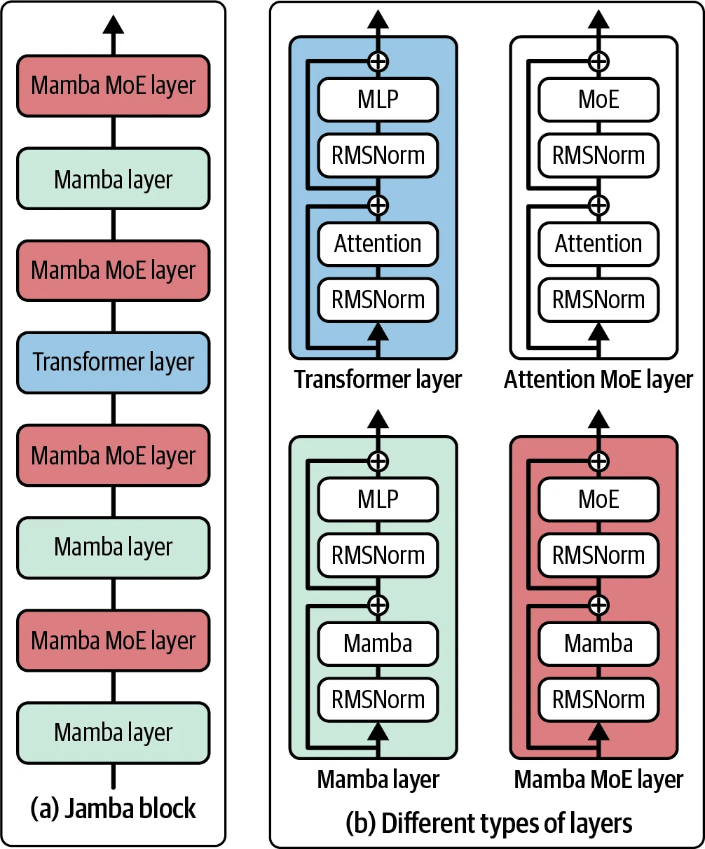Figure 2-7. Transformer, Mamba, and Jamba blocks

None of these has displaced the transformer at frontier scale as of the book's writing, but hybrids are a live research direction, and an engineer should know that "no KV cache" is their main selling point.

Model size and scaling

Parameters, tokens and FLOPs

Three numbers describe a model's scale.

Parameters. A 7B model has seven billion learnable weights. Parameters set memory needs: at 16-bit precision each parameter is two bytes, so a 7B model needs about 14 GB just for weights, and a 70B model about 140 GB, before the KV cache. Parameter count is a poor proxy for compute in sparse models: a mixture-of-experts model such as Mixtral 8x7B has about 46.7 billion parameters total but activates only about 12.9 billion per token, so it runs at the cost of a 13B dense model while holding the knowledge of a larger one.

Training tokens. Dataset size is reported in tokens because tokenization differs across models. Llama 1 trained on 1.4 trillion tokens, Llama 2 on 2 trillion, Llama 3 on about 15 trillion. Tokens seen is not the same as unique tokens: some data is repeated for several epochs.

FLOPs. Floating-point operations measure the compute spent. A useful approximation for dense transformers is training FLOPs ≈ 6 × N × D (N parameters, D tokens): a forward pass costs about 2 FLOPs per parameter per token and the backward pass about twice that. GPT-3 (175B, 300B tokens) used about 3.1 × 10²³ FLOPs; Llama 3.1 405B used about 3.8 × 10²⁵.

Turning FLOPs into wall-clock time means dividing by hardware throughput times utilization. An H100 delivers on the order of 10¹⁵ dense FP16 FLOP/s on paper; real training achieves a model FLOPs utilization (MFU) of roughly 35 to 50 percent. At that rate the Llama 3.1 405B run took about two months on roughly 16,000 H100s, which at cloud prices is tens of millions of dollars for a single training run before any failed experiments.

Scaling laws and Chinchilla

Loss decreases smoothly and predictably as parameters, data and compute grow. The question is how to split a fixed compute budget between a bigger model and more data.

Aspect	Kaplan et al. (OpenAI, 2020)	Hoffmann et al., "Chinchilla" (DeepMind, 2022)
Finding	Loss is more sensitive to model size than data; grow N faster than D	N and D should grow in roughly equal proportion
Rule of thumb	Big models, comparatively little data	About 20 training tokens per parameter for compute-optimal training
Result it explained	GPT-3: 175B parameters on 300B tokens	Chinchilla: 70B parameters on 1.4T tokens matched or beat Gopher (280B) at the same compute
Serving cost	High, because the model is large	Lower for the same quality

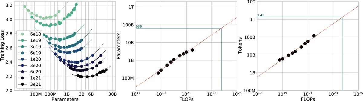Figure 2-8. Scaling laws for predicting optimal parameters and training data

Chinchilla showed that a generation of models had been undertrained: the same compute would have bought a smaller, better model that is also cheaper to serve. The current practice goes further. Compute-optimal is not inference-optimal: if you will serve billions of requests, a smaller model trained far past the Chinchilla point saves more in serving than it costs in training. Llama 3 8B was trained on roughly 1,900 tokens per parameter, almost a hundred times the Chinchilla ratio, precisely for that reason.

Two caveats. Scaling laws predict pre-training loss, and lower loss does not translate linearly into downstream usefulness. And they assume the data exists; past a certain scale it does not.

Scaling extrapolation

Training a frontier model is a one-shot experiment, so you cannot sweep hyperparameters (learning rate, batch size, initialization) on it. Scaling extrapolation (or hyperparameter transfer) trains many small models, fits how the optimal hyperparameters move with scale, and extrapolates to the large run. Parameterizations such as µP (maximal update parameterization) are designed so that the optimum stays fixed across widths, which Cerebras-GPT and others used to transfer settings from millions to billions of parameters. The practical point: a single large run's recipe is the output of hundreds of cheap runs.

Bottlenecks: data and electricity

Data. Villalobos et al. (Epoch AI) projected that the stock of high-quality public human-written text would be exhausted by training runs sometime between roughly 2026 and 2032 if growth continued. Three compounding problems: the web is increasingly filled with model-generated text, which recycles existing patterns rather than adding information; publishers and platforms are blocking crawlers or signing exclusive licensing deals, shrinking the open stock; and the most valuable remaining data (proprietary documents, private conversations, scientific data) is not public. Responses include multimodal data, synthetic data with verification, and the data-quality work above.

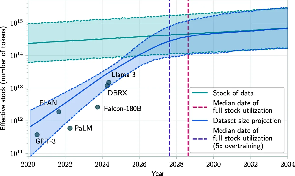Projected growth of training datasets against the stock of public human-generated text: the internet is being consumed faster than it grows

Electricity. Data centers already consume an estimated 1 to 2 percent of global electricity. Compute can grow with more chips only as long as there is power and cooling to run them; grid connections, not GPUs, are now the binding constraint for several hyperscalers, and regions have paused new data-center permits. Scaling by another two orders of magnitude on the current trajectory is an energy problem as much as a chip problem.

Post-training

A pre-trained model is optimized for completion, not conversation. Ask it a question and it may continue with another question, because that pattern is common in its data. It also reproduces the toxicity, bias and misinformation of the web. Post-training fixes both: it teaches the conversation format and steers outputs toward what people want. The usual picture is two steps.

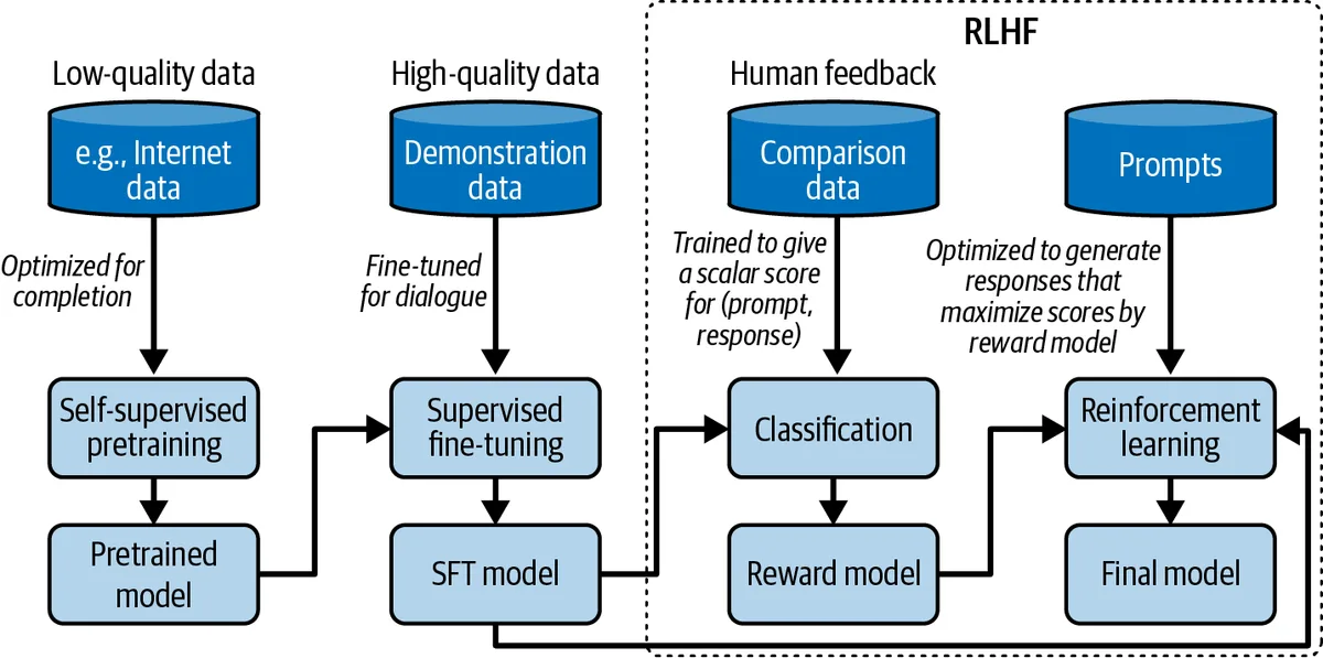Figure 2-10. The overall training workflow with pre-training, SFT, and RLHF

The community's informal image captures the division of labor: pre-training builds a vast, alien completer; SFT gives it a face that talks like an assistant; RLHF paints on the smile. The underlying model's knowledge comes almost entirely from pre-training, which for InstructGPT consumed up to 98 percent of total compute and data. Post-training is small by comparison but decides what you experience.

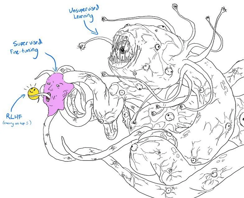The popular picture of post-training: a pre-trained model, a supervised-finetuned face, and an RLHF smile on top

Supervised finetuning

Supervised finetuning (SFT) continues next-token training on demonstration data: (prompt, response) pairs showing how the model should respond. The responses are written by labelers who are selected for the ability to write good answers, which makes this data expensive, typically a few dollars to tens of dollars per example for general tasks and more for expert domains.

InstructGPT (2022) used about 13,000 demonstration prompts covering generation, open QA, brainstorming, chat, rewriting, summarization, classification and extraction, with generation and open QA dominating. Llama 2's chat models used about 27,500 demonstrations. Studies such as LIMA showed that around a thousand carefully chosen examples can teach the format, though more and more diverse data continues to help, and many labs now generate demonstrations with stronger models and have humans verify them.

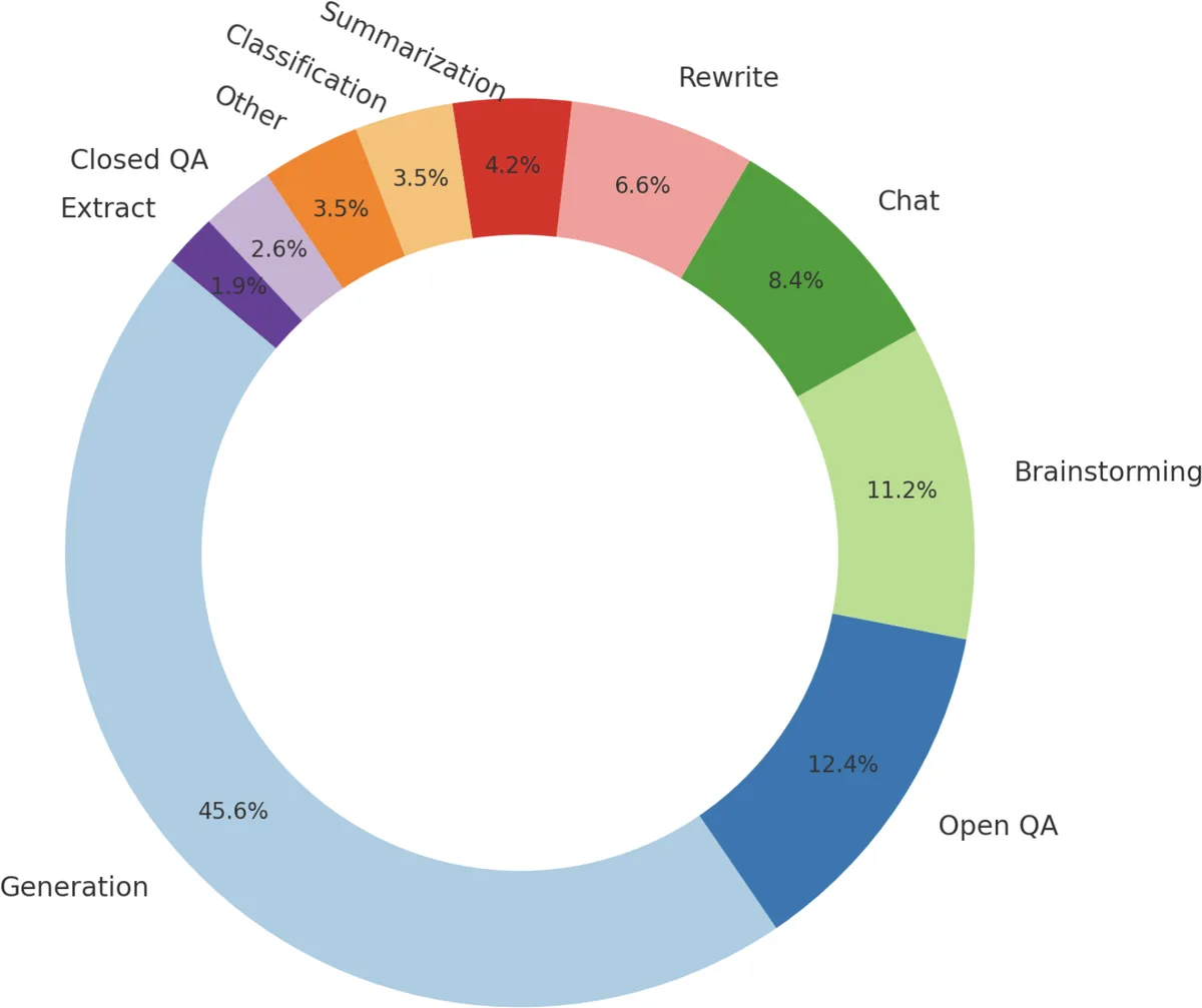Figure 2-12. Distribution of prompts used to finetune InstructGPT

SFT teaches what a good response looks like. It does not directly teach the model which of two plausible responses is better, and writing perfect demonstrations for every subjective task is impossible. That gap is what preference finetuning fills.

Preference finetuning with RLHF

For most tasks it is far easier for a person to say which of two responses is better than to write the best response. RLHF (reinforcement learning from human feedback) uses that cheaper signal in three stages.

Stage 1: collect comparison data. For each prompt the SFT model produces several responses and labelers rank them or choose pairwise winners, often with guidelines about helpfulness, honesty and harmlessness. InstructGPT's labelers worked in a side-by-side interface; the comparison set covered about 33,000 prompts.

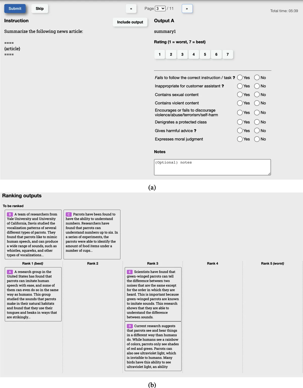Figure 2-13. OpenAI labeler UI for creating comparison data

Stage 2: train a reward model. The reward model (RM) takes (prompt, response) and outputs a scalar score. It is usually initialized from the SFT model (or a smaller model; InstructGPT used a 6B RM for a 175B policy) and trained so that the preferred response scores higher than the rejected one. The loss is a pairwise logistic loss: minimize −log sigmoid(r(winning) − r(losing)) over the comparison pairs. The RM is a learned proxy for human judgment and inherits labeler biases, including a well-documented preference for longer answers.

Stage 3: optimize the policy with PPO. The SFT model becomes the policy of a reinforcement-learning loop. It samples responses, the RM scores them, and Proximal Policy Optimization (PPO) updates the weights to increase expected reward. A KL-divergence penalty against the frozen SFT model keeps the policy from drifting into degenerate text that scores well with the RM but reads badly, a failure called reward hacking. Without the penalty the policy exploits RM blind spots; with too strong a penalty it barely changes.

RLHF is powerful but operationally heavy: four large models in memory (policy, reference, RM, value function), unstable training, many hyperparameters. That cost motivated simpler alternatives.

DPO and RLAIF

Direct Preference Optimization (DPO, 2023) observes that the RLHF objective with a KL penalty has a closed-form optimal policy, so the reward can be rewritten in terms of the policy itself. That turns preference finetuning into a classification loss on (prompt, chosen, rejected) triples: increase the relative log-probability of the chosen response and decrease the rejected one, scaled by how far the policy has moved from the reference. No reward model, no sampling loop, no PPO. DPO is more stable and cheaper, and Llama 3 used it for its final alignment stage. Its weakness is that it only learns from the fixed preference set; RLHF keeps sampling fresh responses and can discover better ones.

RLAIF (reinforcement learning from AI feedback) replaces or augments human labelers with a model that applies written principles, as in Anthropic's Constitutional AI (2022). It scales preference data cheaply and consistently, at the risk of baking the feedback model's biases into the policy. Most production pipelines now mix human and AI feedback.

What post-training costs you

Post-training can be skipped (base models are released for people who want to do their own), and it is a trade-off, not pure gain. Heavily aligned models refuse legitimate requests, hedge, and grow verbose; the loss in raw capability is sometimes called the alignment tax. Post-training also changes probability calibration, which is why perplexity is a worse quality signal for chat models than for base models (Chapter 3), and, as discussed below, it can teach a model to answer confidently beyond its knowledge.

Sampling

A model does not output text; it outputs a probability distribution over its vocabulary for the next token. Sampling is how you pick a token from that distribution, repeated until a stopping condition. The settings you choose change the output as much as the prompt does.

From logits to probabilities

For each step the output layer produces one logit per vocabulary token: an unnormalized score. Softmax converts logits into probabilities: p_i = exp(z_i) / sum_j exp(z_j). Picking the highest-probability token every time is greedy decoding; drawing from the distribution is sampling. APIs often expose logprobs (log of the probabilities) for the chosen and top alternative tokens, which is the cheapest confidence signal you can get from a model and is useful for classification, data filtering and detecting low-confidence answers.

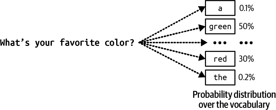Figure 2-14. To generate the next token, the language model computes probability distribution

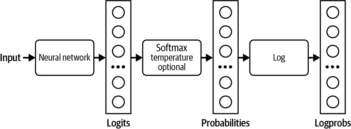Figure 2-17. How logits, probabilities, and logprobs are computed

Temperature

Temperature T divides the logits before softmax: p_i = exp(z_i / T) / sum_j exp(z_j / T). Lower temperature sharpens the distribution toward the top token; higher temperature flattens it. Two candidate tokens with logits 1 and 3 illustrate the effect.

Temperature	P(token with logit 1)	P(token with logit 3)	Behavior
0.5	0.02	0.98	Near-deterministic
1.0	0.12	0.88	The model's learned distribution
2.0	0.27	0.73	Flat, many unlikely tokens become plausible

Temperature 0 is treated as greedy decoding. Values around 0.7 are common for creative writing; 0 to 0.3 for extraction, classification and code. Temperature does not add knowledge; it only trades consistency for diversity.

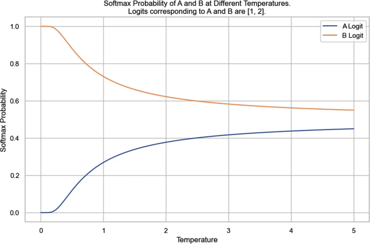Figure 2-16. Softmax probabilities at different temperatures

Top-k and top-p

Top-k keeps only the k highest-logit tokens and renormalizes. It also saves compute: softmax over 50 to 500 tokens is cheaper than over a 100,000-token vocabulary. Its weakness is that k is fixed while the distribution's shape is not. When the model is confident, k = 50 keeps 49 junk candidates; when it is uncertain across hundreds of reasonable tokens, k = 50 cuts good ones.

Top-p (nucleus) sampling keeps the smallest set of tokens whose cumulative probability reaches p (typically 0.9 to 0.95), so the candidate set shrinks when the model is confident and grows when it is not. Min-p is a newer variant that drops tokens whose probability is below a fraction of the top token's probability. In practice top-p is the adaptive truncation most people use; top-k is left at a large default.

Parameter	Low setting	High setting	Typical range	Use
Temperature	Deterministic, repetitive	Diverse, risk of incoherence	0 to 1 (up to 2 in some APIs)	Overall randomness
Top-k	Very narrow	Permissive	1 to 100	Hard cap on candidates, compute saving
Top-p	Narrow and adaptive	Nearly full distribution	0.9 to 1.0	Adaptive truncation

Stopping conditions

Generation ends when the model emits an end-of-sequence token, hits the max tokens limit, or produces a configured stop sequence. The max-tokens limit is a cost and latency guard, not a formatting tool: a response cut off mid-JSON is malformed. Set it from the longest valid output you expect plus margin, and treat a length finish reason as an error to handle.

Test-time compute: best-of-N and voting

You can buy quality at inference by generating several candidates and choosing among them, a family the book calls test-time compute.

• Best-of-N. Sample N responses, score each with a reward model or verifier, return the best. This is the inference-time cousin of RLHF's reward model and needs no weight updates.
• Majority voting (self-consistency). For tasks with a short extractable answer, sample N reasoning chains and return the most common final answer. Different reasoning paths reaching the same answer is strong evidence.
• Logprob selection. Choose the candidate with the highest average per-token log-probability. Cheap, but biased toward bland outputs.
• Beam search. Keep the B highest-scoring partial sequences at each step. Classic in translation, rarely used for chat because it favors generic text.

Sampling more outputs improves the chance that at least one is correct, and the gain continues over many orders of magnitude of samples for code and math where a verifier exists. The cost is linear in N, so this is a lever for high-value, low-volume requests, and DeepMind and others have argued that spending compute this way can beat spending it on a bigger model.

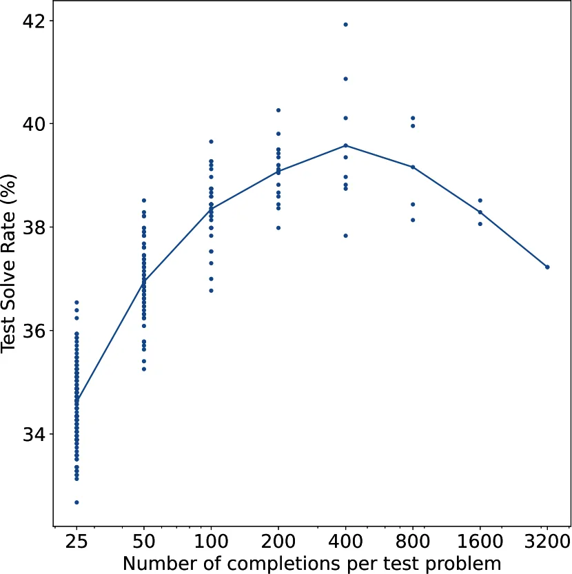Figure 2-19. Sampling more outputs led to better performance

Structured outputs

Downstream code needs JSON, SQL, a class label or a schema-conformant object, not prose. Four approaches, in rising order of reliability and engineering cost:

Approach	Mechanism	Reliability	Cost and limits
Prompting	Describe the schema, give examples, ask for "only JSON"	Medium; models still add prose or drop fields	Free; degrades on complex schemas
Post-processing	Parse, then repair recurring mistakes (missing bracket, trailing comma, markdown fences)	Medium-high for known error patterns	Cheap; models repeat the same mistakes, so fixers pay off
Constrained sampling	At each step mask logits of tokens that would violate a grammar or JSON schema	Very high; output is valid by construction	Needs a grammar per format, modified inference, may hurt content quality
Finetuning	Train on examples in the target format, or add a classifier head for fixed labels	High; model internalizes the format	Training data and ops; locked to the trained format

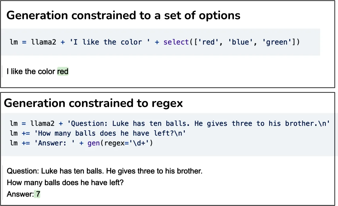Figure 2-20. Using guidance to generate constrained outputs

Constrained sampling (also called guided or grammar-based decoding) is how libraries such as Guidance, Outlines and provider "JSON mode" or structured-output features guarantee validity: a finite-state machine or grammar tracks which tokens are legal next, and illegal tokens are masked before softmax. It guarantees shape, not correctness: a schema-valid object can still contain a hallucinated value. It can also degrade quality when the grammar forces a token the model considers unlikely, and keeping a grammar for every output format is real engineering work.

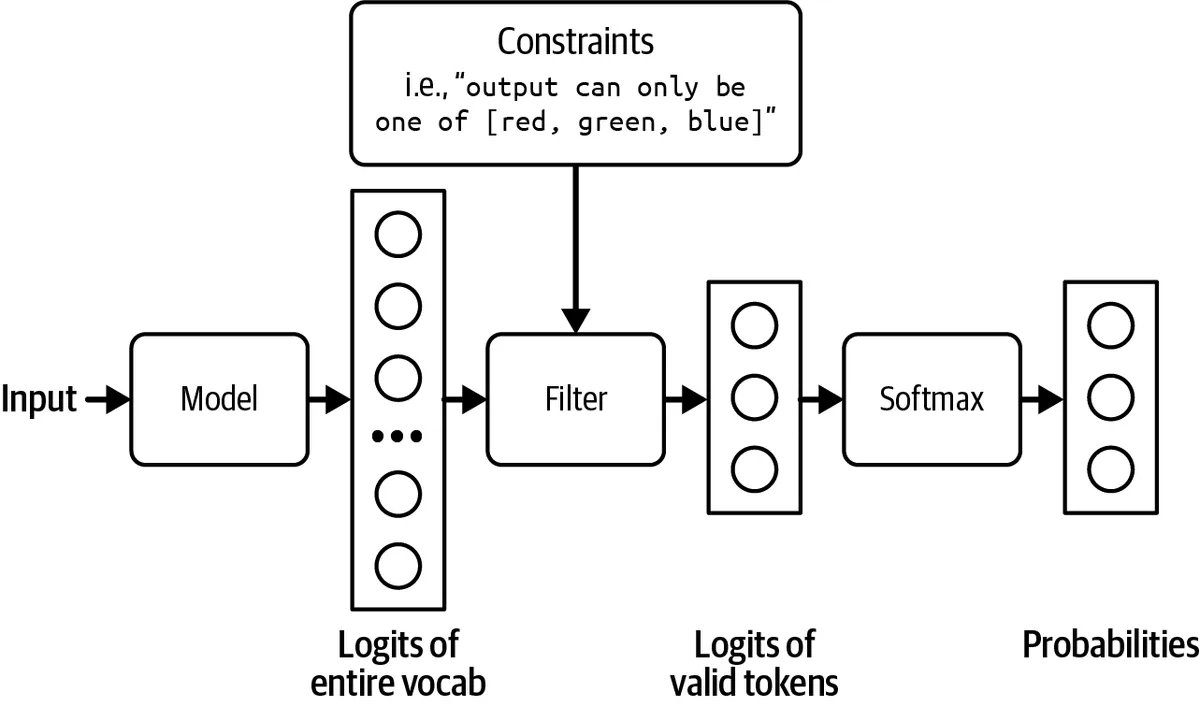Constrained sampling filters the logits to the tokens allowed by the grammar before softmax picks the next token

For pure classification, finetuning with a classifier head replaces the vocabulary output layer with a small head over the desired labels, so the model can only ever answer with a class. This is cheaper at inference than generating label text and sidesteps parsing entirely.

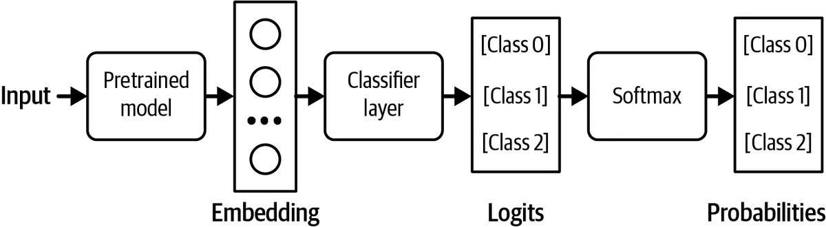Figure 2-22. Adding a classifier head to your base model

The probabilistic nature of AI

Sampling makes outputs probabilistic by design. That is the source of creativity and also of the two failure modes you will spend the most engineering time on.

Inconsistency

Same input, different outputs. At any temperature above zero the same prompt yields different responses. Even at temperature zero, outputs are not guaranteed identical: floating-point nondeterminism across hardware, batching, and silent provider model updates all change results. An essay-grading prompt run twice can return a 3 and then a 5.

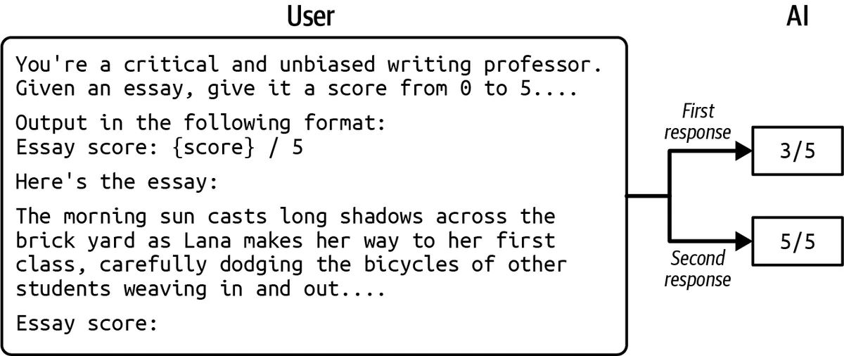The same essay-scoring prompt, run twice, gets a 3 and a 5: models are inconsistent even on identical input

Slightly different input, very different outputs. Reordering few-shot examples, changing one word, or adding a trailing space can flip an answer. This makes prompt evaluation statistical: a change that "worked" on three examples proves nothing.

Mitigations are system-level rather than model-level:

• Cache responses for identical inputs where freshness allows.
• Fix temperature at 0 and pin a seed where the API supports it, and pin model versions.
• Constrain outputs (schemas, classifier heads) so variation cannot leak into the structure.
• Evaluate with many samples and report distributions, not single runs.
• Use voting or best-of-N when a wrong answer is expensive.

Hallucination

A hallucination is fluent, confident content that is not grounded in fact or in the provided context: invented citations, fabricated API parameters, wrong arithmetic defended with made-up reasoning. It is the main blocker for deploying models in high-stakes settings. The book presents two hypotheses for why it happens; they are complementary and lead to different mitigations.

Hypothesis 1: self-delusion. Proposed by Ortega et al. at DeepMind (2021), this says a model cannot distinguish between tokens it was given and tokens it generated itself. Once it has emitted a claim, it conditions on that claim as if it were fact, and subsequent tokens build on it. Zhang et al. (2023) called the effect snowballing: a model that wrongly states 9677 is not prime will go on to invent a factorization, while a fresh session asked directly about the same number answers correctly. The initial error was a sampling accident; everything after it was the model being consistent with itself.

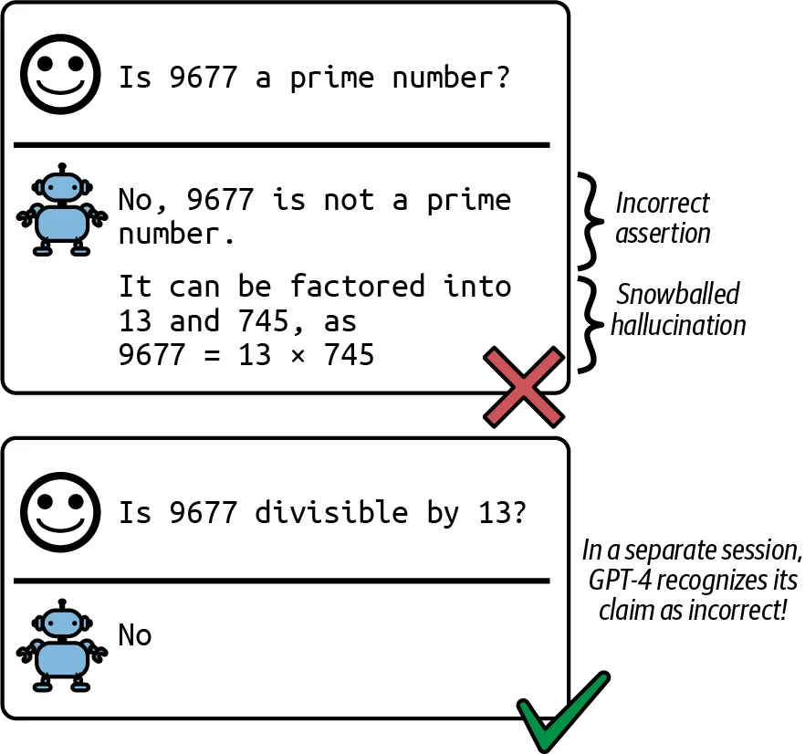A snowballed hallucination: once the model claims 9677 is not prime it invents a factorization, while a fresh session answers correctly

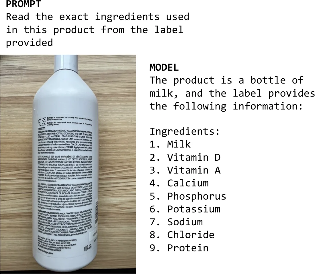Figure 2-24. An example of self-delusion by LLaVA-v1.5-7B

Mitigations under this hypothesis: reinforcement learning that rewards grounded answers over fluent ones, prompting the model to answer only from provided context and to cite it, asking it to verify or re-derive a claim before committing (the fresh session got it right), and structuring long generations so that early mistakes can be caught before the model elaborates on them.

Hypothesis 2: mismatched internal knowledge. Argued by Leo Gao and later by John Schulman (2023), this says hallucination is taught during post-training. Demonstrations are written by labelers who know things the model does not. Training on them teaches the model to produce confident, complete answers in that style whether or not it has the underlying knowledge. The SFT data is correct; the lesson it teaches ("always answer like this") is wrong for a model with gaps. One study found that a model trained with both SFT and RLHF hallucinated more than its SFT-only counterpart, consistent with preference training rewarding confident completeness.

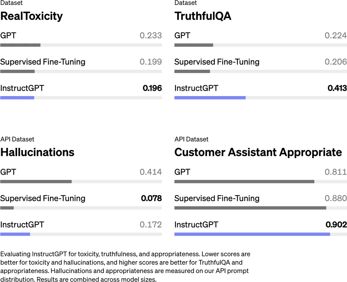Figure 2-26. Hallucination is worse for the model that uses both RLHF and SFT

Mitigations under this hypothesis: include demonstrations where the right answer is "I don't know", have labelers verify that the model could plausibly know what the demonstration asserts, and design reward functions that penalize a confident wrong answer more than a hedge and penalize a hedge more than a correct answer, so the policy learns to express calibrated uncertainty.

Neither hypothesis gives an application developer a switch to flip, which is why the application-level defenses recur throughout the book: retrieval so the facts are in the context, verification steps, citation requirements, constrained outputs, and human review proportional to stakes. Chapter 4 covers how to measure hallucination; Chapter 6 covers retrieval.

Design trade-offs: choosing settings and approaches

Decision	Options	Guidance
Model size	7B to 70B open weights, or hosted frontier	Smaller models trained on more tokens are often the best quality per dollar at inference; size alone is a weak signal, training tokens and post-training quality matter more
Architecture	Dense transformer, MoE, hybrid SSM	MoE gives large-model quality at small-model per-token compute if you can hold the weights in memory; SSM hybrids when context length and memory dominate
Temperature	0 to 0.3, 0.7 to 1.0	Low for anything parsed by code or graded for correctness; higher only for deliberate diversity
Truncation	Top-p 0.9 to 0.95, top-k large	Top-p adapts; leave top-k as a safety cap
Structured output	Prompt, repair, constrain, finetune	Prompt plus repair until failure rates matter; constrained sampling when validity must be guaranteed; classifier head for pure labels at volume
Quality vs cost at inference	Single sample, best-of-N, voting	Spend N on high-stakes, verifiable, low-volume requests; never as a substitute for fixing the prompt or data
Alignment level	Base model, instruct model	Base when you finetune heavily or need raw completion; instruct for everything else
Hallucination defense	Retrieval, verification, abstention, review	Pick by stakes: retrieval and citations first, verifier model second, human review for irreversible actions

Interview angle

• Walk me through how a transformer generates one token. The prompt is tokenized and embedded; each block applies causal self-attention (queries against cached keys and values of earlier tokens, softmax-weighted sum of values) then an MLP, with residuals and normalization; the final hidden state is projected to logits over the vocabulary; sampling picks a token; its key and value are appended to the KV cache and the loop repeats until EOS.
• Why is time to first token different from time per output token? Prefill processes all prompt tokens in parallel and is compute-bound, so TTFT grows with prompt length. Decode generates one token at a time and is bound by memory bandwidth, dominated by reading weights and the KV cache per step, so TPOT depends on model size and context length but not on prompt parallelism.
• What is the KV cache and why does long context cost so much? It stores every earlier token's key and value vectors so attention does not recompute them. It grows linearly with sequence length and with layers and heads, consuming GPU memory that would otherwise serve more requests, which is why long-context requests lower throughput and raise cost.
• Explain Chinchilla and why Llama 3 ignored it. Chinchilla says for a fixed training budget, about 20 tokens per parameter minimizes loss. Llama 3 8B trained on roughly 100 times that because the goal was inference efficiency: a smaller model served billions of times saves more than the extra training costs. Compute-optimal is not deployment-optimal.
• Compare RLHF and DPO. RLHF trains a reward model on human comparisons then optimizes the policy with PPO against that reward with a KL penalty; it can explore new responses but is expensive and unstable. DPO rewrites the same objective as a classification loss directly on preference pairs, removing the reward model and RL loop; it is simpler and stable but learns only from the fixed preference data.
• What goes wrong without the KL penalty in RLHF? The policy exploits the reward model's blind spots, producing text that scores high but is degenerate or off-distribution. The KL term keeps the policy near the SFT model so the reward model's judgments remain valid.
• A product manager asks why the model gives different answers to the same question. What do you say, and what do you do? Sampling draws from a distribution, and even at temperature 0 hardware and provider changes add nondeterminism. Fix temperature and seed, pin the model version, cache identical requests, constrain output structure, and evaluate changes across many samples instead of one.
• Why do models hallucinate, and how would you reduce it in a RAG system? Two hypotheses: self-delusion (the model treats its own earlier tokens as fact and snowballs) and mismatched internal knowledge (post-training taught it to answer confidently beyond what it knows). In RAG: put the facts in context, instruct answering only from context with citations, verify citations exist, allow abstention, use a verifier or judge on high-stakes answers, and measure groundedness.
• How would you guarantee valid JSON from a model? Prompt with the schema and examples, repair known failure patterns, and for guarantees use constrained decoding (grammar or JSON-schema masking of logits) or a provider's structured-output mode. Remember it guarantees shape, not truth, and set max tokens so output is never truncated mid-object.
• When is best-of-N worth it? When you have a reliable verifier or reward model, the request is high-value and low-volume, and a wrong answer costs more than N times the inference. Code with tests and math with checkable answers are the classic cases.

Pitfalls and misconceptions

• "Parameter count tells you quality." Training tokens, data quality and post-training matter as much. A 7B model trained on 15T tokens beats older 65B models; an MoE's total parameters overstate its per-token compute.
• Reading Chinchilla as a deployment rule. It optimizes training compute. For a model you will serve at scale, overtrain a smaller model.
• Thinking temperature 0 means deterministic. It means greedy, which is usually but not always reproducible. Floating-point order, batching and model updates all introduce variation.
• Using top-k and top-p as creativity knobs. They truncate the tail; temperature reshapes the distribution. Tuning all three at once makes effects impossible to attribute.
• Treating max tokens as output control. It is a cost guard; hitting it truncates output. Control length with the prompt and watch the finish reason.
• Assuming post-training adds knowledge. Knowledge comes from pre-training. SFT and RLHF change format, style and preference alignment, and can increase hallucination by rewarding confident completeness.
• Believing constrained decoding fixes hallucination. It fixes syntax. The values inside the valid structure can still be wrong.
• Expecting equal quality across languages. Training data is roughly half English; low-resource languages get worse answers, more tokens per sentence and higher cost.
• Blaming the model for inconsistency instead of the system. Caching, seeds, pinned versions, schemas and multi-sample evaluation are the engineer's job.

Key terms

Term	Meaning
Common Crawl	Nonprofit web crawl of two to three billion pages a month; the raw material behind C4, The Pile, RefinedWeb and most open pre-training corpora
Seq2seq	Encoder-decoder RNN architecture whose fixed hidden-state bottleneck and sequential processing the transformer replaced
Attention	Mechanism where each token's query is scored against all keys and the softmax weights combine the values
Query, key, value	Three learned projections of each token used in attention: what I look for, what I offer to match, what I contribute
KV cache	Stored keys and values of earlier tokens so decode steps do not recompute them; grows linearly with context
Prefill and decode	The parallel prompt-processing phase and the sequential token-generation phase of inference
Transformer block	Attention module plus MLP with residuals and normalization; models stack dozens of them
Mixture of experts (MoE)	Sparse architecture that routes each token to a few expert MLPs, so active parameters are a fraction of total
State space model (SSM)	Recurrent architecture family (S4, Mamba) with constant memory per token, offered as a transformer alternative
FLOPs	Floating-point operations; training cost is about 6 × parameters × tokens for dense transformers
Chinchilla scaling law	Compute-optimal training uses roughly 20 tokens per parameter; many earlier models were undertrained
Model FLOPs utilization (MFU)	Fraction of theoretical hardware throughput achieved in training, typically 35 to 50 percent
Supervised finetuning (SFT)	Post-training on (prompt, response) demonstrations to teach the conversation format
Reward model	A model trained on human comparisons to score a response; the proxy objective in RLHF and the selector in best-of-N
PPO	Proximal Policy Optimization, the RL algorithm used to update the policy against the reward model with a KL penalty
Reward hacking	The policy exploiting reward-model blind spots to score well with poor outputs
DPO	Direct Preference Optimization: a classification loss on preference pairs that removes the reward model and RL loop
RLAIF	Preference feedback generated by a model following written principles instead of, or alongside, humans
Logits and logprobs	Unnormalized scores over the vocabulary and the log of their softmax probabilities
Temperature	Divisor on logits before softmax; lower sharpens, higher flattens the distribution
Top-k, top-p, min-p	Truncation rules that drop unlikely tokens before sampling
Test-time compute	Spending more inference (best-of-N, voting, verification) to improve a single answer
Constrained sampling	Masking tokens that would violate a grammar or schema so output is valid by construction
Snowballing hallucination	A model elaborating on its own earlier mistake because it cannot tell generated tokens from given facts

Further reading

• AI Engineering, Chapter 2 (Chip Huyen, O'Reilly, 2025). Companion resources: https://github.com/chiphuyen/aie-book
• Vaswani et al., "Attention Is All You Need" (2017): https://arxiv.org/abs/1706.03762
• Hoffmann et al., "Training Compute-Optimal Large Language Models" (Chinchilla, 2022): https://arxiv.org/abs/2203.15556
• Kaplan et al., "Scaling Laws for Neural Language Models" (2020): https://arxiv.org/abs/2001.08361
• Ouyang et al., "Training language models to follow instructions with human feedback" (InstructGPT, 2022): https://arxiv.org/abs/2203.02155
• Rafailov et al., "Direct Preference Optimization: Your Language Model is Secretly a Reward Model" (2023): https://arxiv.org/abs/2305.18290
• Bai et al., "Constitutional AI: Harmlessness from AI Feedback" (2022): https://arxiv.org/abs/2212.08073
• Holtzman et al., "The Curious Case of Neural Text Degeneration" (nucleus sampling, 2019): https://arxiv.org/abs/1904.09751
• Gu and Dao, "Mamba: Linear-Time Sequence Modeling with Selective State Spaces" (2023): https://arxiv.org/abs/2312.00752
• Zhang et al., "How Language Model Hallucinations Can Snowball" (2023): https://arxiv.org/abs/2305.13534
• Villalobos et al., "Will we run out of data? Limits of LLM scaling based on human-generated data" (2022, revised 2024): https://arxiv.org/abs/2211.04325
• Grattafiori et al., "The Llama 3 Herd of Models" (2024), for a documented frontier training run: https://arxiv.org/abs/2407.21783
• Chip Huyen, "Generation configurations and sampling strategies" (2024): https://huyenchip.com/2024/01/16/sampling.html